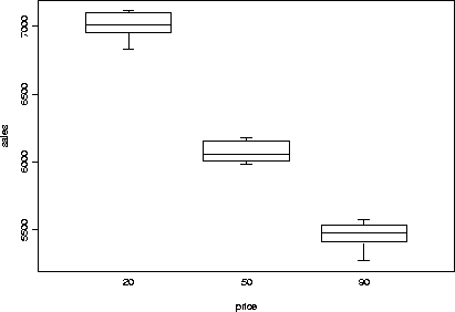
We can illustrate the one-way analysis of variance using the sales data:
402 > attach(salesdata)
402 > sales205090 _ salesdata[((price==20)|(price==50)|(price==90)),]
402 > sales205090$price _ factor(sales205090$price)
402 > table(sales205090$price)  # There are 11 months of sales at each price
 20 50 90
 11 11 11

402 > view(sales205090$price)

      structure(.Data = c(1, 2, 3, 1, 2, 3, 1, 2, 3, 1, 2, 3, 1, 2, 3,
      1, 2, 3, 1, 2, 3, 1, 2, 3, 1, 2, 3, 1, 2, 3, 1, 2, 3), .Label =
      c("20", "50", "90"), class = "factor")

402 > plot.factor(sales205090,style.bxp="old")

402 > sales.aov _ aov(sales ~ price,data=sales205090)
402 > anova(sales.aov)
Analysis of Variance Table

Response: sales

Terms added sequentially (first to last)
          Df Sum of Sq Mean Sq  F Value Pr(F)
    price  2  13332276 6666138 895.2989     0
Residuals 30    223371    7446
402 >  13332276/( 13332276 +  223371 )  # calculate R^2
[1] 0.9835219
This tells us that the ``price'' variable explains much of the
variability in the ``sales'' data, but isn't very informative about
details, like what the mean sales was at each price level, etc.
To obtain this, we need to think about the model in a different way. In ANOVA notation, we would write the model (1) as

where i=1, 2 or 3, depending on whether the price was 20, 50 or 90, and j indexes the 11 observations at each price level.
Nomenclature:
 is called the overall mean or grand mean
 ,
,  and
and  are called ``effects''.
Just to be confusing, they are also called ``contrasts.''
We can add one linear constraint to take away the overparametrization. The usual one for the ``grand means plus effects'' model is to make the effects sum to zero:

The  can then be estimated with the model.tables()
function:
402 > model.tables(sales.aov,type="effects")
Refitting model to allow projection
Tables of effects

 price
    20     50     90
 826.3 -106.6 -719.7
402 > sum(scan())        # verify that the alpha's sum to zero
1:  826.3 -106.6 -719.7
4:
[1] -1.136868e-013
An alternative parameterization with just three parameters is to take
out the intercept and just estimate the mean sales for each price
level, this is called the cell means model:

Again, we can estimate the cell means with model.tables():
02 > model.tables(sales.aov,type="means")
Refitting model to allow projection
Tables of means
Grand mean

 6185

 price
   20   50   90
 7011 6078 5465
Let's compare these results with fitting the model ``by hand'' using lm().
402 > lmsales _ sales205090$sales
402 > lmprice _ sales205090$price
402 > p20 _ ifelse(lmprice==20,1,0)
402 > p50 _ ifelse(lmprice==50,1,0)
402 > p90 _ ifelse(lmprice==90,1,0)
402 > sales.lm _ lm(lmsales ~ p20 + p50 + p90)
Error in lm.fit.qr(x, y): computed fit is singular, rank 3
Dumped
402 > # oops, forgot to delete a column
402 > sales.lm _ lm(lmsales ~ p50 + p90)
402 > summary(sales.lm)

Call: lm(formula = lmsales ~ p50 + p90)
Residuals:
    Min     1Q Median    3Q   Max
 -194.8 -55.67 -4.224 78.53 113.8

Coefficients:
                 Value Std. Error    t value   Pr(>|t|)
(Intercept)  7010.8662    26.0170   269.4728     0.0000
        p50  -932.8187    36.7936   -25.3528     0.0000
        p90 -1545.9577    36.7936   -42.0171     0.0000

Residual standard error: 86.29 on 30 degrees of freedom
Multiple R-Squared: 0.9835
F-statistic: 895.3 on 2 and 30 degrees of freedom, the p-value is 0

Correlation of Coefficients:
    (Intercept)     p50
p50 -0.7071
p90 -0.7071      0.5000
Actually, when lm() sees a factor variable in a
regression, it will construct dummy variables automatically, but
unfortunately it then transforms the X matrix to make the columns
orthogonal; we will learn more about SPLUS's coding of dummy variables
later.