Adding a Line

The function abline adds a line of the form y = a + b*x to a plot. It also has an lty= field to allow different line types (dashed, dotted, etc.).

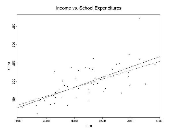
Let's add two lines to the plot of income and school expenditures, one including Alaska and the other not. We can find these lines using regression (explained in the handout on models). The first command below says `` SE70 modelled by PI68'' and the second says ``SE70 modelled by PI68 using all points except the 50th''.

> lm(SE70 ~ PI68)
Call:
lm(formula = SE70 ~ PI68)

Coefficients:
 (Intercept)       PI68
    17.71003 0.05537594

Degrees of freedom: 51 total; 49 residual
Residual standard error: 34.9384
> lm(SE70 ~ PI68, subset=-50)
Call:
lm(formula = SE70 ~ PI68, subset = -50)

Coefficients:
 (Intercept)       PI68
    40.56264 0.04747211

Degrees of freedom: 50 total; 48 residual
Residual standard error: 29.93981

Now we can use the first equation to plot a solid line (line type 1, the default), and the second to plot a dotted line (line type 2).

> abline(17.71003, 0.05537594, lty=1)
> abline(40.56264, 0.04747211, lty=2)

As you can see, the slope is smaller when Alaska is removed from the model, but the two lines are very similar.