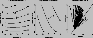
Figure: Selected Store Profit Maps for Premium versus Store Brands
To illustrate the national versus store brand price gap we plot the expected profit function in the first two panels of Figure 8 for two particular stores under a moderate prior. These stores were chosen since they represent the extremes in the slope of the profit contours for these tiers across all the stores. The horizontal axis represents the price index of the store brands, and the vertical axis represents the price index of the premium brands. These price indices show proportional price movements of all the products within the group. In this figure, the prices of the national brands are held constant. The actual average prices of the premium, national, and store brands are about $2.85, $2.30, and $1.70, respectively, during the time span we consider. This yields a price gap of 40% between the premium and store brand tiers.

Figure: Selected Store Profit Maps for Premium versus Store
Brands
The center point (1,1) of the left panel in figure 8 corresponds to the expected profits from the current strategy for store 6, which would be $39,280. The retailer is interested in moving to the more profitable areas, which are located in the upper half of the graph. The directional profit gradient is represented by a vector emanating from the current pricing strategy and shows the direction of the most profitable pricing changes. On this graph the best point is (.8,1.2), which would decrease store brand prices to 80% of their current levels (.8) and increase the premium brands by 20% (1.2). This pricing strategy would result in an increase in profits of $48,760 a year or a 24% increase.
This plot suggests that the optimal solution lies outside the
range under consideration. This result is not unexpected, given our
justification for this model is based on approximation grounds to the
true demand function under present operating conditions. Therefore, our
model will hold only approximately for the neighborhood around the
current pricing strategy. Since our model implicitly assumes no change
in present operating conditions other than prices, we must consider the
possibility of consumer and competitor responses outside the context of
our model. Experimental data would seem to support our contention that
price swings of  10% are plausible for our model, while larger
price swings may not be.
The micro-marketing effect is expressed as the change in slope of the contour lines between these two stores. In store 6 the best direction to head on this profit map is to increase the price for the premium brands and reduce the store brand prices slightly. This results in an increase in the price gap between the premium and store brands. In store 58 the best direction is to increase the prices of both tiers, with the price of the store brands increasing at a faster rate. This results in a decrease in the premium versus store brand price gap. (The best point on store 45's profit contour map is the upper right-hand corner which would result in a 26% increase in profits.) Notice that while the upper left quadrant in store 6 represents a profit increase, for store 58 this would result in a profit decrease.
There are several effects that are driving these results: changes in own-price elasticities, substitution between the tiers, and differences in profit margins for these products. Store 6 is more price sensitive (i.e., higher category elasticity), which means that the own-price elasticities are larger and there is a greater price response for the private labels. Since the impact of the premium brands on the private labels is large, by decreasing the price of the store brands we will experience a quantity demand increase for the store brands. Although the asymmetry between the premium brands and the store brands means that the store brand price decreases will not substantially affect the premium tier sales.
To further depict the price movements for each of the 83 stores,
we plot the directional gradients in the third panel of figure 8. The
axes of this panel are the same as above, although only the first
quadrant is plotted. Notice that the directional profit gradients of
stores 6 and 58 correspond with the extreme vectors in this third panel.
The solid 45 line holds special significance since it denotes
the division between increasing and decreasing the price gaps between
the tiers. The length of the line segments designating the gradients is
scaled by the probability that the angle of the vector is greater than
45
 , or less than 45
 if the vector is below the
45
 . Notice that we are quite confident of whether to increase
the price gaps, and the evidence is fairly strong for four stores that
the price gaps should be decreased. The distribution in profit
gradients illustrates the dispersion of price response across stores.