 Go to spoken version
Micro-marketing refers to the customization of price, promotion, product assortment, and service to the store-level, rather than adopting uniform marketing policies for all stores. Historically there has been a drive by retailers to consolidate operations into large regional or national chains due to large economies of scale in managing their stores (eg., purchasing and distribution). Unfortunately the benefits of a neighborhood store catering to local tastes has been curtailed. However, recent advances in technology and more competitive environments has resulted in a growing interest by large regional and national retailers to differentiate their stores by better serving their customers at a neighborhood level.
There are many possible applications of micro-marketing to retailing problems. It may refer to a retailer carrying a different assortment of products in each of its stores, i.e., Target decides not to carry winter items in its southern outlets. Secondly it may refer to different promotional schedules across stores. For example, Ames Department Stores may follow different promotional and advertising policies in different regions of the northeastern United States. Finally it can also refer to a retailer charging different prices in each store. It is this final form of micro-marketing that we will concentrate upon in this paper. Certainly all these aspects of the problem provide for interesting directions for study, we concentrate upon pricing due to its importance and flexibility to the retailer. The primary focus of this research will be to show that these micro-marketing pricing strategies are profitable and suggest how they can be implemented. The data used in this paper considers how Dominicks Finer Foods (DFF), a major Chicago area supermarket retailer, could customize its pricing policies to reflect neighborhood differences in tastes and purchasing patterns.
Our study begins by considering previous micro-marketing research by Hoch et al. (1995). They show that significant differences in store price elasticities exist at a category level. These results suggest that overall category price changes between stores could be profitable. Overall price changes offers only a slight glimpse into the much richer set of micro-marketing pricing strategies that are available. Price-quality tier research (Blattberg and Wisniewski 1989) would suggest that price gaps between quality tiers would be an interesting direction for study. For example is it the case that the price gap between national and private labels is greater for some stores than others? Moreover can we carry this line of questioning to its lowest level: How should store-level demand variations affect an individual product's price?
Throughout this paper we will concentrate on micro-marketing from the retailer's perspective. This will position our problem in its natural decision-theoretic context. This contrasts with the usual analysis that would stop with the measurement of store-level price elasticities. A driving force in the formulation of our demand model and pricing strategies will be the consideration of the information set that is available to the retailer. As part of this study we apply our model to store-level scanner data for the refrigerated orange juice category. Our purpose is not only to seek a unique optimizing solution to the pricing problem, but also to consider directions of price changes which result in higher profits.
At the core of this problem is the measurement of price sensitivity for every product in each store. We will take a general approach to modeling brand competition by constructing systems of demand equations for each category. While this approach avoids imposing specific substitution patterns on a category, it results in a huge number of parameters. This creates a formidable estimation problem since it becomes difficult to reliably measure store-level differences in price sensitivity. To improve our estimates, Bayesian shrinkage techniques are employed. Formally this is a random coefficient model embedded within a hierarchical Bayesian framework. This paper makes use of Gibbs sampling, a recent advance in statistical computing, to compute estimates of the exact finite-sample posterior distribution.
A similar application of hierarchical bayesian models in a marketing context was presented by Blattberg and George (1991). A contribution we make is the use of demographic variables as a source of heterogeneity in the parameters. Also our model shrinks the store parameters towards a linear relationship instead of a single central tendency. This component of our study represents a long line of marketing research identifying covariates for market segmentation (Webster 1965, Montgomery 1971, Frank et al. 1972, Blattberg et al. 1978, Bawa and Shoemaker 1987 & 1989). An innovation presented here is that this segmentation can occur at the store-level. Additionally we allow for a full error covariance matrix instead of assuming independent errors across the products, formulate a different method for parameterizing the priors, and evaluate the effects of the prior in terms of its impact on both the posterior distribution of the parameters and profits.
The plan of the paper is as follows. In Section 2, we discuss the modeling of the retailer's store-level demand and profit functions. Section 3 considers the estimation of these store-level demand models in a Hierarchical Bayesian model. We present the supermarket scanner data to which our model will be applied and discuss issues related to variable selection in Section 4. Section 5 addresses model estimation. In Section 6, we deal with how store-level differences influence the retailer's profit function. Section 7 enlarges this discussion by moving toward simpler and more general pricing strategies. We consider the implications of these findings in Section 8.
This paper takes a general approach to modeling brand competition by constructing a system of demand equations for each store. Each product is modeled as an equation in which its movement is a function of its own price, cross effects of price changes from all other products in the category, and its feature and deal status for that week. This approach avoids imposing a specific substitution pattern on the category. Although a specific market structure could be used to induce a more parsimonious substitution pattern, such as a macro-logit model, or other constraints on the cross-elasticity matrix (Allenby 1989). We avoid imposing these constraints in order to avert rigid forms on market structure, since we wish to allow for the possibility that the market structure is changing from one store to another.
We will model the system of demand equations facing an individual store using a semi-log functional form. This demand system can be expressed as:
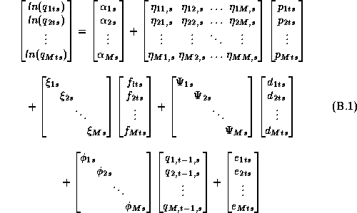
Where  , and
, and  are
movement, price, feature, and deal respectively. The subscript i
denotes the product number, t is week, and s is store. The vector of
error terms,
  through
  , follows a multivariate normal
distribution with mean 0 and covariance matrix
  .
The off-diagonal
parameters of the feature, deal, and lag movement variables are zero.
Equation 2.1 can be expressed in matrix form:

Note that the number of parameters in this system can be very large since a typical category has between 10 and 100 products.
The system in 2.1 does not include measures of income, cross-category prices, and competitor prices. In our empirical application it was not possible to obtain accurate measures of these variables. An important assumption in the demand specification for an individual category is that utility for that category is weakly separable from other categories, both in the same store and across stores. Additionally we assume substitution between categories is relatively low. Therefore, as long as the average price changes of the other categories and weekly changes in income are relatively small, we can interpret the coefficients (weighted by their price) as uncompensated price elasticities.
The retailer's weekly expected profit function is implicitly defined by the demand system in 2.1:

where  is the retailer's cost
of product i in week t for store s. The complete problem to the
retailer's optimal pricing solution includes pricing, competitor
responses, promotional strategy (eg., feature, display, in-store
couponing, shelf placement, etc.), and costs (eg., forward buying,
inventory control, administrative and selling costs, etc.). We will
concentrate upon pricing, which will yield only a partial solution to
this global problem. A primary reason for concentrating on price is
that it is one of the most important variables under the retailer's
control. A more pragmatic concern is that we have only limited
information about promotional and competitive pressures. Additionally,
we argue that the incremental costs to setting up a micro-marketing
strategy are small. Since we will only consider changes in prices,
these changes should be easy to incorporate into existing scanner
pricing systems.
The formulation of full demand systems in the previous section
avoids enforcing specific substitution patterns, but results in a huge
number of model parameters. We can see that this presents a formidable
estimation problem. The two extreme solutions to this estimation
problem are to allow each store to have its own model or to pool all
stores together. The individual store models can be estimated using
standard least squares (LS) techniques.![]() . In this setup every store would be
independent from the others and has its own set of parameter values.
Unfortunately, the individual store models generally have poor
predictive ability and the standard errors of the parameter estimates
are too large to be useful for deriving pricing strategies. At the
other extreme, the pooled chain-level model has fair predictive ability,
but it does not account for any of the heterogeneity across stores since
it would assume that the parameter values are identical for all stores.
Estimation for the pooled model using standard LS theory could easily be
applied by stacking all the stores into a single system.
. In this setup every store would be
independent from the others and has its own set of parameter values.
Unfortunately, the individual store models generally have poor
predictive ability and the standard errors of the parameter estimates
are too large to be useful for deriving pricing strategies. At the
other extreme, the pooled chain-level model has fair predictive ability,
but it does not account for any of the heterogeneity across stores since
it would assume that the parameter values are identical for all stores.
Estimation for the pooled model using standard LS theory could easily be
applied by stacking all the stores into a single system.
To improve the individual store estimates, we will borrow information from across the stores using a hierarchical Bayesian model (Lindley and Smith, 1972; Smith 1973). We can think of our demand systems forming a random coefficient model, in which the parameters for each store are draws from an underlying distribution. The central tendency of this distribution represents the average chain-wide effects. The deviation of a parameter from the chain-wide mean can be decomposed into a systematic and random effect. This systematic component is related to the store's demographic and competitive characteristics. The random component is a unique store-specific effect. Recent work by Rossi, McCulloch, and Allenby (1994) on hierarchical Bayesian models has also employed demographic variables to explain consumer heterogeneity in a household-level probit model.
To make the procedure as general as possible we rewrite our
demand system in SUR form:![]()

Here the s subscript denotes an individual store, and the dimension of the y vector is M brands by T weeks. In rewriting the model we have stacked the vector of observations for each brand:
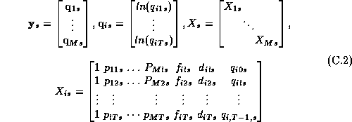
Note that  in equation 3.2 refers to the vector of log
movement for a given brand over all weeks, whereas
  in
equation 2.2 it refers to the vector of log movement across all brands
for a given week. To complete this stage, we also specify natural
conjugate priors using a Wishart distribution on the error covariance
matrix
  :
:

The second stage refers to the hyper-distribution from which the parameters for each store are drawn:

Where all the parameters from a store's demand system ( ),
have been stacked into a single vector:

diag(Q) denotes a vector of the diagonal elements from a matrix Q. To
complete this second stage, we include a prior distribution on the
covariance matrix of the second stage  :
:

The motivation for
representing  with a prior distribution instead of specifying it
directly is to allow for some uncertainty in the amount of commonalities
across stores.
The relationships between the demand parameters and the demographic
and competitive variables are contained within the  term. We will assume that a consumer's utility function can be
separated along the lines of the price-quality tiers (Blattberg and
Wisniewski 1989). This allows us to place a specific structure upon the
relationship between the demand parameters and demographic variables.
Furthermore each tier will be approximately modified by a linear
function of demographic variables which can be motivated by differences
in household production functions (Becker 1965). We can show that the
cross-price sensitivities within a tier and between tiers have the same
demographic relationships using Lewbel's results (1985). Also, we make
a further modification by allowing the own-price coefficients and
feature coefficients to have their own demographic relationships within
each tier. A formal presentation of these arguments is given in
Montgomery (1994).
We can express the linear relationships between the individual coefficients and the demographics as:
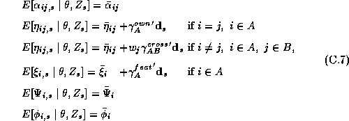
where  is the vector of demographic and competitive
variables for store s,
  denotes the corresponding
coefficients, and
  denotes the average market share for product
j
denotes the average market share for product
j![]() . Both of these vectors are
. Both of these vectors are
 . A and B denotes the set of products within
price-quality tiers A and B, in our application we have three
price-quality tiers. To give the barred constants the
interpretation as chain-wide averages, the
  vectors are
standardized with zero means
  .
.
To illustrate the effects of these common demographic relationships
within the price quality tiers, consider the cross-store variation of
the own-price sensitivities. This  vector will have three
separate demographic effects:
  , which correspond with the
premium, national, and store brand tiers respectively. The change in
own-price sensitivity across the stores will have a common demographic
component for all brands within a tier. For example, all three premium
brands will share the same demographic predictor. However, the
individual brands are not restricted to this relationship, since there
will be some random variation about this linear demographic predictor.
Our primary purpose in having these common demographic effects within
each tier is to reduce the number of demographic relationships to a
reasonable number. An alternate specification would have allowed each
parameter to have its own demographic relationship, however this would
have resulted in a highly parameterized model that could present
estimation difficulties. An additional effect of this specification
will be to induce some shrinkage of the changes in the parameter
estimates across stores towards a common tier effect for each store.
This will result in a more limited pattern of shrinkage than Blattberg
and George (1991), which would also shrink parameter estimates within a
store towards one another.
Since all these relationships are linear, we can easily incorporate
them into the  matrix. We can partition
  and
and  into constants and demographic components:

Where the vector of chain-wide averages in the hyper-distribution is:

and the relationships with the demographic and competitive variables are given by:

The  matrix is composed of 1's and 0's and represents the
constant vectors and therefore is the same for each store. In our model
we let each
  have its own intercept, hence
  is the
identity matrix with order 192. If certain elements are to be
``shrunk'' toward one another then the corresponding elements in a
particular column are both set to 1, and the other elements set to 0.
Since the demographic data vector for each store is the same for
all the parameters, the construction of the  matrix can be
simplified using the following relationship:

The  matrix is
constructed in an analogous manner to
  , except that it summarizes
the systematic relationships. In our analysis the
  matrix has 15
columns: three columns for the own-price sensitivities (one in each
tier), nine columns for the cross-price sensitivity terms (a full
three by three interaction between the tiers), and three columns for
the feature price coefficients (one in each tier). To illustrate this
matrix consider the column which corresponds to the premium own-price
sensitivities, if the parameter is a premium own-price sensitivity
then the element is set to 1, otherwise the element is 0.
Geometrically this allows for every coefficient to have its own
intercept, but there is a common slope for the own-price elasticities
inside each quality tier.
The third stage of our model expresses the prior on the hyper-parameters:

In our specification we will employ a diffuse third
stage prior. But an informative prior on  would specify prior beliefs about
chain-wide tendencies or demographic and competitive effects on
parameter variation. The W matrix is included to make the
specification of this prior more flexible.
The analyst must supply the following parameters and data:

Our priors on the error covariance matrices,  , and mean
of the hyper-distribution,
  , are chosen to be diffuse
relative to the sample. The mean and degrees of freedom for the
prior on
  are:
are:

The parameters of the prior on our hyper-distribution are:

The most crucial prior will be on  , which reflects
the strength of the commonalities across the stores. Notice that in our
case the number of stores is less than the dimension of
  .
Therefore to form a proper posterior distribution, we will need to have
an informative prior. Although as more information is added (more weeks
of observations), the individual estimates of the
  's will
dominate this prior in deriving the posterior distribution of
  and
and  .
.
The motivation of the parameterization of our prior on  is to shrink our parameter estimates somewhere between the pooled and
individual LS estimates. For simplicity we set to
  a
diagonal matrix. To allow for proper scaling of the different
coefficients we set the diagonal elements equal to the product of the
variance least squares estimates from the individual store models,
 , and a scaling parameter,
  :
:

where p is the dimension of  (or 192, i.e., 12
equations with 16 parameters each). We also set
  . The
relationship between
  and
and  can be
seen by examining the mean and covariance matrix of this prior
distribution:
  and
and  .
.
We are primarily concerned with parameter variation across stores.
We do not try to shrink the parameters within a store (i.e., across
products) closer to each other. Therefore, we let each store and brand
have their own intercepts. Also to avoid a great deal of shrinkage in
the constants we set the scaling parameters of these parameters to one
or  , whichever is greater.
We set the scaling parameters for the other parameters equal.
Therefore,
  for constants and
  for all other
parameters (if k>1, then
  for constants also). This setup
for the hyper-distribution contrasts with Blattberg and George (1991)
who are primarily concerned with improving individual brand estimates of
price elasticities by shrinking all brand price sensitivity parameters
toward a common central tendency across all brands and stores.
If the scaling parameters are small (say .1) then our prior states
that the standard deviation of store-specific random variation of our
estimates will be 10% of those of the LS estimates. (Notice that
parameter variation will also induced by the demographics.) The
degenerate case of k=0 with  behaves similarly to the
pooled estimates, since there will be no cross-store variation in the
store parameters. If k=0 with
  we will mimic a
model with direct demographic and competitive interactions. An
empirical Bayes prior or one which reflects moderate commonalities would
set k to unity. If the scaling parameters are large (k=5) then our
prior states that the standard deviation of our estimates will be five
times those of the LS estimates. Which implies that our stores will have few
commonalities and there will be little shrinkage. As
  our estimates converge to those of individual store models, although in
practice values of k>10 will approximate this result. An assessment
of this prior on the predictive ability of the model is given in section
5, while its influence on profits is discussed in section 6 and 7.
The data used in this paper represents a unique single source dataset. Its uniqueness is a result of its size and the depth of information about movement, prices, promotion, profit margins, and competition. The data was collected from Dominick's Finer Foods (DFF) as part of the Micro-Marketing Project at the University of Chicago (Dreze, Hoch, and Purk 1993). DFF is a major supermarket chain in the Chicago metropolitan area with a 20% market share of supermarket sales. There are three different types of information used in this paper, each coming from different sources and discussed in the following sub-sections. The types of data collected here are readily available to supermarket retailers.
Store-Level Scanner Data: DFF provided weekly UPC-level scanner data for all 88 stores in the chain for up to three years. The scanner data includes unit sales, retail price, profit margin, and a deal-code. Out of these 88 stores, five have limited historical data, so we concentrate on the remaining 83 stores. To verify the correctness of the data, comparisons across stores and categories were made for each week. Certain weeks in which the integrity of the data was in doubt were removed from the sample. Also one brand was introduced in the early part of the data (Florida Gold), and another brand (Citrus Hill) is removed in the later part. Consequently we consider the middle 121 weeks of the sample period (June 1990 through October 1992), to avoid introduction and withdrawal effects.
There are 33 UPCs in the category. In order to a create a more manageable number of products we create twelve aggregates from the original UPC level data that have similar pricing and promotional strategies. The UPCs within a product aggregate differ only by flavoring, additives, or packaging (eg., regular, pulp, or calcium). The price of the aggregate is computed as a price index (i.e., an average weighted by market share) over all the UPCs that comprise the aggregate. The movement of the aggregate is computed as the sum of the movement (standardized to ounces). Prices within each aggregate are approximately proportional, therefore little pricing information is lost. Moreover we can still speak about profit maximization since we assume the relative prices of the items within an aggregate are fixed.
Summary statistics for average weekly prices, gross profits, and market shares across stores for the twelve aggregates are listed in Table 1. There is a natural division of products into three price-quality tiers: the premium brands (made from freshly squeezed oranges), the national brands (reconstituted from frozen orange juice concentrate), and the store brands (Dominick's private label). There is quite a bit of disparity in prices across the tiers, which leads to large differences in wholesale costs, even though the profit margins appear similar. An initial indication that store differences are present is the variation of market shares across stores. Dominick's 64 ounce OJ brand has an average market share of 13.3%, but the market shares across stores range anywhere from a minimum of 5.5% to a maximum of 20.6%.
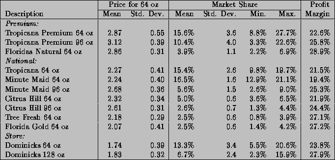
Table 1: Descriptive Statistics for Price, Market Share, and Profit Margins
Promotional Data: Information about feature advertising in weekly newspaper fliers is provided by IRI's Infoscan, which provides an estimate of all commodity volume of a particular UPC that received feature advertisement. IRI collects this data based on a representative sample of approximately 60 stores from throughout the Chicago metropolitan area. The information provided was at an aggregate level for the Dominick's chain and for all other competitors. The aggregation of the competitor information reduces its value for our purposes and is not used. In-store promotion is measured using a deal code provided in DFF's store-level scanner database. The deal-code is a dummy variable which shows whether there was a bonus-buy sticker on the shelf or an in-store coupon. Since these promotional variables are at the UPC level, we create indices of the feature and deal variables for each aggregate similarly to that of price.
Store Trading Area Data (Competitive/Demographic Characteristics): Market Metrics, a leading firm in the use of demographic data, used block level data from the U.S. Census to compute a store's trading area. A store's trading area refers to a geographical area around the store. It is calculated by finding the number of people needed to sustain a given level of sales for this area. Geographical boundaries (such as roads, railroad tracks, rivers, etc.) are considered when this trading area is formed. The demographic composition of the store's trading area is computed by summing up the assigned proportion of each of the U.S. Census blocks within the prescribed trading area.
The selection of variables is guided by a household production framework. For a further discussion of variable selection issues refer to Hoch et al. (1995). A total of eleven demographic and competitive variables are used to characterize a store's trading area. These variables summarize all the major categories of information that are available. Table 2 lists each variable along with their descriptive statistics. The statistics in the table are generated for the 83 stores in our sample. Four of the demographic variables measure general consumer characteristics: the percentage of the population over age 60 (Elderly), percentage of the population that has a college degree (Educ), the percentage of black and Hispanic persons (Ethnic), and the percentage of households with five or more members (Fam-size). The other demographic variables are: log of median income (Income), the percentage of homes with a value greater than $150,000 (House-val), and the percentage of women who work (Work-wom).
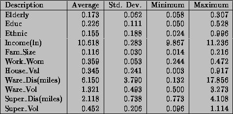
Table 2: Descriptive Statistics for Demographic/Competitive Variables Across Stores
The other four variables measure the competitive environment of the store's trading area. There are two broad types of stores for which we have information: warehouse and supermarkets. The warehouse stores are larger and use an everyday low pricing strategy (EDLP). Other supermarket stores use a high-low pricing strategy (Hi-Lo) similar to Dominick's. We have broken out competitive effects between these two groups since we expect that these two pricing strategies will have different effects. For each group we use two measures of competition: distance (in miles) and relative volume. Distance is doubled in urban areas to reflect poorer driving conditions, which approximates Market Metrics measure of driving times. Relative volume is the ratio of sales in the competitor to that of the Dominick's store. The warehouse competitor variables are computed with respect to the nearest warehouse store, and the supermarket competitor variables use an average of the nearest five competitors.
While the nested structure of the model makes it easy to form the
hierarchical model, estimation is a problem since an exact solution of
the posterior distribution is not known. Even with natural conjugate
priors we are unable to derive exact finite sample results. The
difficulty in deriving the posterior distribution is a result of the
Wishart priors on  and
and  . The analytical solution
which integrates
  out of the joint distribution of
  to derive the posterior distribution is not known. To understand the
difficulty of this problem, we refer the reader to the simpler case of
trying to solve a single stage SUR model (Zellner 1971, pp. 240-6) for
which the analytic solution is not known either. Therefore, we rely
upon numerical procedures to find the solution. Unfortunately the high
dimension of the integral makes it difficult to find a solution using
conventional numerical integration techniques.
There are many techniques that could be applied to give an approximate answer. A simple technique would be to estimate these elasticities in two-stages. We could estimate the store-level systems using LS estimates, and then regress these estimates in a second-stage regression upon the demographics. This is the approach taken in Hoch et al. (1995). The deficiency with this method is its inefficiency. Alternately an estimator based upon a normal approximation could be carried out (see Appendix B).
Since these approximations may be questionable we make use of a new technique in computational statistics known as the Gibbs sampler to estimate the marginal posterior distributions. Due to the hierarchical structure of the model, the solution of the conditional distributions is straightforward. See Appendix A for a solution of the conditional distributions and a description of our implementation of the Gibbs Sampler. An added benefit of the Gibbs draws is that we may compute an estimate of the marginal posterior distribution of the expected profit function. Traditionally the posterior means of the parameter estimates are substituted into the profit function, which means the uncertainty of the parameter estimates is not incorporated into the profit function. Blattberg and George (1992) show that this method does not lead to an optimal pricing solution due to the nonlinearity of the profit function. Therefore, our procedure does not suffer from the drawbacks of the traditional method.
To illustrate the shrinkage effects of the Bayes estimator
discussed in the previous sub-section consider a single parameter, the
own-price elasticity of Minute Maid 64 oz Orange Juice. We will use a
strong prior (i.e.,  ) in this sub-section for expositional
purposes. Our purpose is to contrast the Bayes estimate with those of
the individual LS models. As is customary the point estimates for the
Bayesian model are the means of the marginal posterior distribution.
Figure 1 overlays the estimates from the individual LS store models, the
pooled model, and the Bayesian model.
In this figure the own-price sensitivity estimate is plotted against the predicted parameter using the demographic/competitive information. The open diamonds represent the own-price elasticity for Minute Maid 64 Oz orange juice. The solid diamonds represent the estimates from the Bayesian model. To picture the relationship between these two estimates, a dashed line with an arrow pointing from the LS estimate toward the Bayesian estimate is drawn. The arrow illustrates the idea of shrinking the LS estimate toward some central tendency, which is represented by a solid line. The solid line represents the expected relationship between the store's trading area characteristics and the own-price elasticity of Minute Maid 64 Oz orange juice using the Bayesian model. The pooled estimate is the same for each store, and is represented by a dashed line.
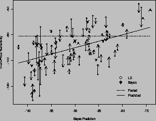
Figure 1: Least Squares versus Bayes Estimates for Minute Maid 64 oz
A positive relationship between the least square estimates and the prediction using the demographic/competitive score can be observed. This relationship is weakened a great deal by purely random estimation error. By using cross-store information and the prior knowledge that stores differ in their relationships to this demographic/competitive score we can estimate this effect with greater precision. If we consider an average store with a demographic/competitive score of zero, then the expected-own price elasticity would be -89.43 with a standard-deviation of 2.08. (Multiplying by the average price of .035 yields an average price elasticity of -3.13.) The pooled model estimate of this parameter is -81.13. By accounting for the heterogeneity that is present in the stores we do not induce a strong bias into the estimate of the central tendency across stores, as in the pooled model.
The Gibbs Sampler can be used to derive estimates of the exact solutions to the marginal posterior distributions. A disadvantage of the Sampler is the computational burden to compute a large number of iterations. Another possible estimator is one based upon a normal approximation, which should perform well for large samples (both weeks and number of stores) and is relatively cheap to compute. To find out the accuracy of the approximation we compare these two estimators under various priors.
If we assume relatively diffuse prior knowledge then the true
estimator converges to a generalized least squares one for each store.
Since the hierarchical model will reduce to individual stores models for
a diffuse prior, we would expect agreement between these two estimators
for relatively weak priors, such as k=5. As the prior is tightened
up, i.e., smaller k values, we would expect that the approximate
estimator may no longer be as good. For expositional purposes we will
plot the marginal posterior distribution of the hyper distribution
( ) that corresponds to the own-price elasticity of Minute-Maid
Orange Juice for the Gibbs and normal estimators in figure 2. We
consider three different priors for each of these parameters: weak
(k=5), moderate (k=1), and strong (
 ) priors. The marginal
posterior distributions for both parameters are very close for the weak
prior (top panels). However as the prior is tightened to a moderate
prior (middle panel) we can discern a noticeable bias in the variance
of the posterior for the normal estimator. In the case of the strong
prior (bottom panel) we find strong biases in both the location and
variance of the normal estimator. For the posteriors of the
hyper-parameters involving the demographic variables these biases are
even more pronounced. However, if our primary goal is to find a point
estimate of the hyper-distribution mean then a normal approximation
seems adequate for weak and moderate priors.
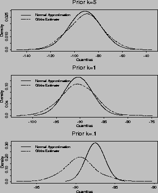
Figure 2: Marginal Posterior Density for Hyper-Distribution of
Minute-Maid 64 oz Own-Price Sensitivity
We have used the Gibbs sampler as a basis for comparison since theoretically it can be shown to be sampling from the marginal posterior if the sampler has converged (Gelfand and Smith 1990 and Gelfand et al. 1990). But the convergence and number of draws of the Gibbs sampler need also be considered, since the Gibbs sampler is a Markov Chain technique. For our implementation we generated 1200 Gibbs iterations according to the algorithm described in Appendix A, using only the final 1100 iterations for estimation of the marginal posterior distributions.
The choice of the number of iterations is influenced by both the
length of CPU time (700 iterations take approximately one day of CPU
time on a Sun Sparcstation 10 Model 41) and the low autocorrelation in
the sampler. In figure 3, we plot the draws from the marginal posterior
distribution of the hyper-distribution ( ) corresponding with the
own-price elasticity for Minute-Maid 64 oz. The Gibbs sampler is
started at the mean of the normal approximation. Since the estimates
are already in the neighborhood of the posterior mean, convergence does
not present a problem. Alternate starting points were also tested, but
the process moves quickly to a neighborhood of high posterior
probability within the burn-in period. The first autocorrelation of the
processes illustrated in figure 3 increases from .04, .21, to .78 as k
decreases from 5, to 1, and to .1. This implies a decreasing
information content of the draws. The rapid convergence and smaller
number of draws follows other studies using similar linear models (see
Blattberg and George (1991) and Gelfand and Smith (1990)).
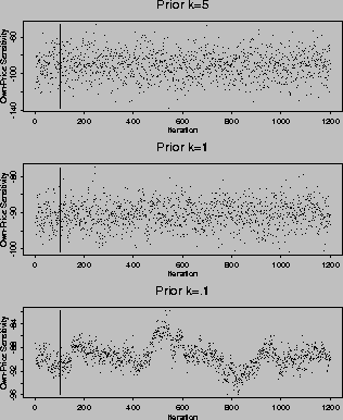
Figure 3: Individual Draws from Gibbs Sampler for Hyper-Distribution
of Minute-Maid 64 oz Own-Price Sensitivity
We have illustrated only the draws from an individual parameter,
but our real concern is the joint convergence of all parameters. To
monitor the joint convergence of the process we look at not only other
individual parameters, but also the trace of  and
and  .
The first autocorrelation of the trace of
  is less than .07
for k equals to 5 and 1, but increases to .30 for
  . The first
autocorrelation of the trace of is always less than .15. Our only real
concern is the high first autocorrelation in the vector
  , which increases
from .06, .50, to .97 for k equals to 5, 1, and .1. Clearly for weak
and moderate priors there should be little concern over the number of
draws, although for stronger priors more draws are desirable.
The specification of the prior distribution of  is
critical to our problem. This prior characterizes our prior beliefs
about the commonalities across stores, which decides the shrinkage of
the non-systematic store component of the parameters toward the central
tendency. To validate the choice of our prior and better understand its
influence on the posterior we will perform out-of-sample predictions.
These predictions are performed for a series of prior specifications
ranging from strong to weak prior beliefs about the communality across
stores (i.e., k from .01 to 10). (See Appendix A for a discussion of
the parameterization of this scaling parameter.) The sample is divided
into two halves, each with roughly 60 weeks. Since we are primarily
concerned with point estimates using the mean of the posterior
distribution, we employ the estimates derived from a normal
approximation (Montgomery 1994).
The average MSE for in- and out-of-sample predictions for various
values of k is plotted in figure 4. For large values of k, say 10,
the average out-of-sample MSE is close to that of the individual LS
models for each store (.424). As k decreases the out-of-sample
predictive ability increases, for k=1 and  we have a 19% (.351)
and 24% (.324) decrease in MSE respectively. The pooled model shows a
decrease in out-of-sample MSE by only 12% (.380), which shows that by
allowing for some heterogeneity in the store parameters can improve the
out-of-sample predictive ability. Another alternative model is a
clustered store model. Here we formed three clusters of stores based on
the demographics and competitive variables. Then we estimate separate
models for each cluster. The MSE of the predictions from this clustered
model are similar to the pooled model (.383).
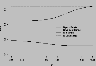
Figure 4: Comparison of Average MSE for various priors
Even though the out-of-sample predictions are improving, the
in-sample fit worsens for smaller values of k, but that is to be
expected since the LS estimates by definition minimize the in-sample
MSE. For k=1 and  we have a 6% (.162) and 23% (.189) increase
of in-sample MSE over the individual LS models (.153). Also, notice a
relative increase in the MSE from the in-sample to the out-of-sample
period. One reason for this increase is that the MSE is a biased
measure of the average error variance. If we ignore the
heteroskedasticity in the residuals, and simply adjust the MSE by the
number of observations (57,612) and by the number of parameters
(15,936), then the MSE should be multiplied by a factor of 1.38 to
enable a comparison between the in- and out-of-sample MSE. A second
reason is that since we are dealing with a period of several years,
long-run price swings may result in poorer predictions. Finally pricing
and shelving experiments were conducted during this sample that were
uncharacteristic of in-sample periods and may diminish predictive
accuracy.
These results show that the out-of-sample predictions can be improved by avoiding the homogeneity assumptions involved in pooling. This improvement does not sacrifice the in-sample fit of the model as does the pooled model. The increased predictive ability of the Bayesian models does show there is support in the data for strong or moderate priors in commonalities of cross-store parameter variation. However, the discriminatory power of the data using our out-of-sample MSE criterion is not great in identifying whether these commonalities are strong or moderate. Moreover, this improved prediction does not imply that a particular prior is correct.
The parameters from each store model can be thought of as a draw
from an underlying normal hyper-distribution with mean  and covariance matrix
  . In this section we describe
the posterior mean for this hyper-distribution using a strong prior
(i.e.,
  ). We have selected this prior, since it is most
insightful to consider common store tendencies when we are willing to
express strong prior beliefs that they exist. Table 3 lists the price
elasticity matrix computed at the average prices. Along with the
central tendency is a measure of the standard deviation of the random
store-specific variation, i.e., the diagonal elements of the posterior
mean of
  . (Note
  gives the standard deviation of
the hyper-distribution and not the standard error of the estimates.)
For example Minute Maid 64 oz has an average own-price elasticity of
-2.84, with a standard deviation of .31 for store specific fluctuations.

Table 3: Posterior Mean ( ) and Standard Deviation (
 ) of the
Hyper-Distribution for the Cross-Price Elasticity Matrix using Average
Prices and prior k=.1
The cross-price elasticity matrix is a 12 x 12 matrix, and summarizes information about substitution between products induced by price changes. The average of the own-price elasticities (diagonal elements) and cross-price elasticities (all off-diagonal elements) is -2.75 and .18 respectively. Also smaller sizes have larger own-price elasticities than larger sizes. Florida Gold is the most own-price sensitive brand with an own-price elasticity of -3.67. This is probably the result of the brand not engaging in a significant amount of national advertising, and not establishing a great deal of brand equity.
The mean and standard deviation of the constant, deal, lag, and
feature coefficients in the hyper- distribution are provided in table 4.
Since the dependent variable is the log of movement, the units of these
parameters can be interpreted as percentage changes in movement. The
large posterior standard deviations of the constants show that there is
a great deal of diversity in the intercepts of the demand functions,
which is the result of both preference and store size differences. The
deal coefficients are typically small and dominated by the feature
promotions. The lag coefficients are also very small, except Citrus
Hill 96 ounce. The feature<\A> variables
show strong promotional
sensitivity, although the price discount given on feature must be added
in to compute the full effect of feature promotions. The average
feature coefficient is .60, with the most promotional sensitive brand
being Florida Gold 64 ounce. Feature responses for national brands are
largest followed by the store and then the premium tiers.
Tables 5 and 6 provides the posterior mean and standard error of the
demographic and competitive variable effects upon price and feature for
each of the 15 linear relationships. To illustrate the demographic
relationships consider the effects of household value upon the various
groups of coefficients. There is a positive relationship between the
premium and national own-price sensitivity and household value.
Therefore as the percentage of households in the store's trading area
with a house value of over $150,000 increases, consumers are less
own-price sensitive. The demographic relationships for the store brand
own-price sensitivities are not precisely estimated.
For the cross-price sensitivities there are mixed results. In the
premium tier, increasing household values result in less substitution
between brands within this segment. The same moderating effects of
household values on substitution toward national brands are also
present, as represented by the negative coefficients. For store brands
we see an increase in substitution as household values increase,
although it is difficult to measure a precise effect. The negative
feature coefficients dampen the promotional effects. These effects are
generally consistent with the predicted wealth effect. That is as
household value increases, we would expect people to be less price
sensitive. In addition, price discounts lead to smaller substitution
effects and feature effects will be weaker in areas with higher
household values.
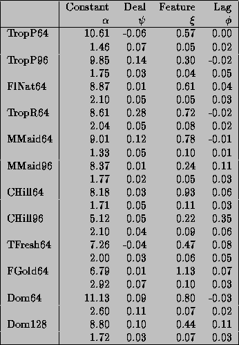
Table 4: Posterior Mean ( ) and Standard Deviation
(
 ) of the Hyper-Distribution for the Other Parameters with a
Strong Prior
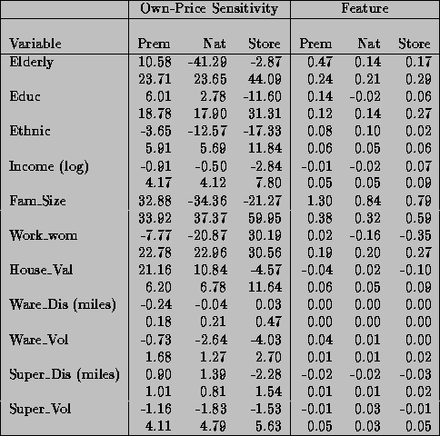
Table 5a: Posterior Mean ( ) and Standard Error of
Demographic and Competitive Effects upon Price and Feature Sensitivity
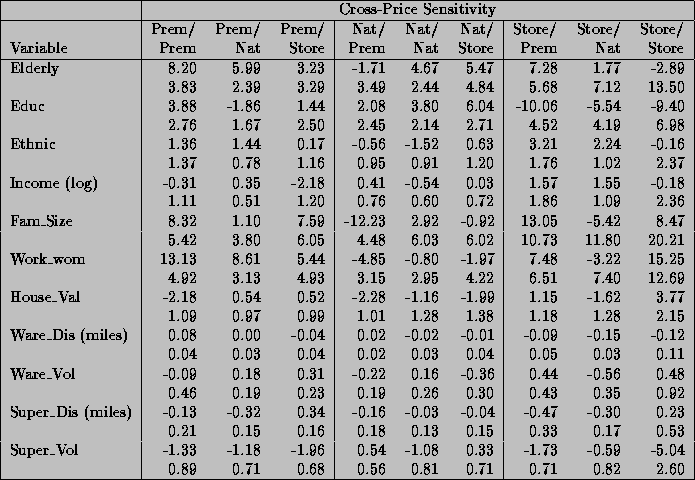
Table 5b: Posterior Mean ( ) and Standard Error of
Demographic and Competitive Effects upon Cross-Price Sensitivity
Micro-Marketing Pricing Strategies
As discussed in the introduction we will concentrate only upon a single component of the retailer's pricing strategy. The problem is that this is still a huge problem, if the retailer wishes to implement a micro-marketing strategy for a single year this would require 51,792 pricing decisions (= 83 stores x 12 products x 52 weeks). Therefore we will simplify the problem to the retailer's everyday pricing problem. In general supermarket retailers determine a base price level and then determine a promotional schedule and price discount. Since promotions can have a strong impact on store traffic and other product purchases we will assume DFF retains its current promotion schedule.
This will allow us to express everyday prices as a function of a base price level and weekly promotional policies. Therefore, the prices for any given week are:

Where  refers to a price multiplier for product i in store
s, and
  is the base price followed by DFF. Notice that if
all
  then prices remain at their current levels. If a
product is featured then we will not change the price of that product.
An additional reason from the retailer's standpoint for
concentrating on the everyday component of the pricing problem is that
75% of profits are made through the sale of products that are not
featured
then prices remain at their current levels. If a
product is featured then we will not change the price of that product.
An additional reason from the retailer's standpoint for
concentrating on the everyday component of the pricing problem is that
75% of profits are made through the sale of products that are not
featured![]() .
.
The retailer is concerned with the present value of total future profit across all stores. We will simplify this by considering only the sum of profits for a given year:

 represents the profits in store s for week t, and
 refers to the total chain profits for week t. The use of a
single year is not limiting, since the solution will generalize if we
assume the retailer has identical profit expectations in future years.
A time-span of one-year instead of a single week was selected to better
reflect the dynamic nature of prices induced by promotional strategies.
Appendix A discusses the
computation of the marginal posterior of the
expected profit function conditional only upon the prices, costs, and
data using the Gibbs sampler.
The findings of previous marketing research (Kumar and Leone 1988, Walters and MacKenzie 1988, and Walters 1991) have shown that intra-store substitution dominates across-store substitution. Furthermore consumers have poor recall of individual product prices (Dickson and Sawyer 1990, Supermarket Business 1992). Therefore we assume that competition between stores is occurring through general price levels and promotional strategies, and does not naively require every price in the store to be identical with its competitor as in a perfectly competitive pricing environment. As our model is currently formulated the retailer has full monopoly powers. Obviously the store's offerings, location, and service are differentiated from its competitors, but it would be extreme to assume full monopoly powers. Therefore we introduce two constraints on the pricing problem to better approximate the current competitive situation: total sales revenue and the average price (weighted by market share) in each store is unchanged from their current levels.
These constraints essentially guarantee that there will not be any change in competitive or consumer response. For a motivation of these constraints on managerial and economic grounds see Montgomery (1994). We do not believe these to be the only viable micro-marketing strategies, but they seem very plausible given the information used in our model. This framework also provides a natural context for evaluating micro-marketing pricing strategies, since any profit gains will solely be the result of store-specific pricing effects and not overall, chain movements.
To assess the incremental benefits on profits of a micro-marketing strategy we employ a uniform pricing strategy as a basis for comparison. A uniform strategy equates the prices of an individual product across all stores, although the prices of different products may vary. A uniform pricing strategy is the antithesis of a micro-marketing strategy, since all stores have identical price vectors. Dominick's could expect gross yearly profits for this category to be around $3.4 million using a uniform pricing strategy.
The profits from the optimal constrained and unconstrained pricing strategies are reported in Table 7 for each prior. The constrained strategy holds average store price and revenues to their values under a uniform strategy. We also add a bound of 10% on any price changes, to guarantee that any solution will be in a relevant range. This bound reflects the price range the retailer was willing to entertain in controlled experiments. These optimal values are computed numerically using the NAG subroutine E04VCF since an analytical solution to the optimal price is not known for this model. The column titled ``Uniform Chain Pricing Strategy'' are those profits earned by the retailer following an identical pricing strategy in each store. Whereas the column titled ``Micro-Marketing Pricing Strategy'' are those earned by the retailer when the price solution for each store is allowed to be store specific. To gain some insight into the spread between the marginal posterior profit distributions, we compute the probability this new strategy will exceed the 90th percentile of the uniform price strategy. The probability of all micro-marketing strategies exceeding a uniform price strategy is greater than .99, which shows these gains will be noticeable after considering the natural variation of the profit distribution.

Table 6: Category Gross Profit Changes under Optimal Pricing Strategies
Using a moderate prior we would realize a .42% increase in gross profits if the retailer moved to a better uniform pricing strategy that did not change average store prices or revenues. The actual price changes implied by this strategy are small. This reflects the difficulty in finding a new pricing strategy that generates more profits than the uniform strategy and retains the current average prices in each store. On the other hand if we allow each store to follow its own pricing strategy than the retailer can realize a 3.46% increase in gross profits. If we were to change the prior and assume that store level differences have greater commonalities, we would expect that micro-marketing profits would increase by 2.74%, while under a weaker prior that assumes fewer commonalities profits would increase by 4.29%.
Lifting off these constraints, but still allowing each store to have its own prices, we could generate a profit increase of 29.08%. If we were to only allow uniform price changes without any constraints we would still increase profits from the current uniform strategy to 26.55%. This 2.53% profit increase from the uniform unconstrained to the micro-marketing unconstrained represents the incremental contribution of micro-marketing. It is purely a micro-marketing effect since no chain-wide price differences occur.
Figure 5 illustrates the effects of the price changes implied by an optimal constrained micro-marketing pricing strategy with a moderate prior. Each boxplot denotes the store-level price changes for each product. To illustrate the effects of these price changes consider Minute Maid 64 Oz. In over 75% of the stores we would want to increase the price of this product. Certain products have very broad ranges in price movements, like Florida Natural in which the prices in some stores are increased by 10% and others are decreased by 10%. Although it is possible for the average price for any particular product across stores to increase, the revenue and average price across products within a store must remain constant due to our constraints.
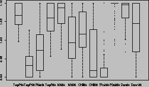
Figure 5: Boxplots of Constrained Optimal Price Changes Across
Stores
In section 5 we discussed the sensitivity to the prior in terms of out-of-sample predictions. In this section we can use a more natural metric, profits, to evaluate the sensitivity of the posterior to changes in the prior. It is clear from Table 7 that the posterior is sensitive to changes in the prior, as our prior becomes weaker the store specific differences grow and we find larger store-level demand differences. Yet whatever the strength of our prior beliefs, we still reach the same substantive conclusions that store-level differences in price sensitivity can be measured and translated into profitable micro-marketing strategies.
The previous section provided a conservative estimate of the profit benefits of micro-marketing pricing strategies. Conservative since no revenue or average price changes were allowed, although we would expect small or even moderate changes in these constraints would be permissible. One difficulty that retailers may have in implementing these types of pricing strategies is the huge data requirements and the complexity of the optimal price calculations. Therefore, it is of interest to consider simplified micro-marketing strategies. This will also help us to gain a better sense of the shape of the profit function. We will begin by considering profits at a product level, move to broader classes of products organized in price-quality tiers, and then onto overall price changes at a store level.
The profit gradient with respect to price provides the direction of steepest ascent in the profit function, i.e., the most profitable direction for unconstrained price changes. Store s's profit gradient is:

The chain profit gradient is the sum of each store's profit gradient evaluated at the same price point.
The posterior distributions for the gradient of the expected category profit function are displayed as boxplots in Figure 6 for three different priors. This plot illustrates a common tendency to increase the prices of each brand except Citrus Hill 96 oz, although the desire to increase prices is strongest for the leading brands. (The dots in the center of the gradient denote the posterior mean and the maximum extent of the whiskers denote the 10th and 90th percentiles.) The gradients have been divided by the total chain profits and the prices are in terms of a percentage change from the current pricing strategy. These adjustments allow us to easily interpret the gradient as the effect of a 1% increase of a product's price on total category profits. Although the gradient yields only an approximation for small price changes.
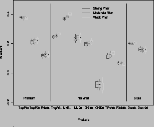
Figure 6: Sensitivity of Chain-wide Profit Gradient
Figure 6 only provides the effects at a chain-wide level, from our micro-marketing perspective what is most interesting are individual store differences. Figure 7 contains the boxplots of the marginal posterior distribution of the Minute Maid 64 oz component of the category profit gradient for selected stores. The variability of the individual store posteriors graphically illustrates the micro-marketing effect. There is still a common tendency to increase the price of this product (a chain-wide effect), although in some stores we would increase the price at a much faster rate than in others. The tightness of the chain distribution is the result of averaging the various store distributions. Notice that there is more dispersion in the posterior for weak priors, while for strong priors the posteriors are tighter.
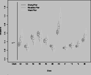
Figure 7: Posterior Sensitivity of Minute Maid 64 oz Category
Profit Gradient
Instead of treating each product separately, we may want to think of price changes across groups of products. One interesting product grouping uses price-quality tiers: premium, national, and store brands. The existence of price asymmetries between price-quality tiers has been well documented (Blattberg and Wisniewski 1989, Kamakura and Russell 1989). One reason to expect these effects to be interesting at the store-level is that we expect income effects to vary across stores because of large disparities in income levels. Following the results of Allenby and Rossi (1991) this implies that there are differences in price asymmetries across stores, which should lead to different price gaps. What makes these gaps even more interesting are the large differences in wholesale costs between these tiers. Dominick's has a 25% wholesale cost difference between the national and store brands in this category.
To illustrate the national versus store brand price gap we plot the expected profit function in the first two panels of Figure 8 for two particular stores under a moderate prior. These stores were chosen since they represent the extremes in the slope of the profit contours for these tiers across all the stores. The horizontal axis represents the price index of the store brands, and the vertical axis represents the price index of the premium brands. These price indices show proportional price movements of all the products within the group. In this figure, the prices of the national brands are held constant. The actual average prices of the premium, national, and store brands are about $2.85, $2.30, and $1.70, respectively, during the time span we consider. This yields a price gap of 40% between the premium and store brand tiers.
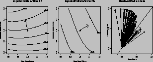
Figure 8: Selected Store Profit Maps for Premium versus Store
Brands
The center point (1,1) of the left panel in figure 8 corresponds to the expected profits from the current strategy for store 6, which would be $39,280. The retailer is interested in moving to the more profitable areas, which are located in the upper half of the graph. The directional profit gradient is represented by a vector emanating from the current pricing strategy and shows the direction of the most profitable pricing changes. On this graph the best point is (.8,1.2), which would decrease store brand prices to 80% of their current levels (.8) and increase the premium brands by 20% (1.2). This pricing strategy would result in an increase in profits of $48,760 a year or a 24% increase.
This plot suggests that the optimal solution lies outside the
range under consideration. This result is not unexpected, given our
justification for this model is based on approximation grounds to the
true demand function under present operating conditions. Therefore, our
model will hold only approximately for the neighborhood around the
current pricing strategy. Since our model implicitly assumes no change
in present operating conditions other than prices, we must consider the
possibility of consumer and competitor responses outside the context of
our model. Experimental data would seem to support our contention that
price swings of  10% are plausible for our model, while larger
price swings may not be.
The micro-marketing effect is expressed as the change in slope of the contour lines between these two stores. In store 6 the best direction to head on this profit map is to increase the price for the premium brands and reduce the store brand prices slightly. This results in an increase in the price gap between the premium and store brands. In store 58 the best direction is to increase the prices of both tiers, with the price of the store brands increasing at a faster rate. This results in a decrease in the premium versus store brand price gap. (The best point on store 45's profit contour map is the upper right-hand corner which would result in a 26% increase in profits.) Notice that while the upper left quadrant in store 6 represents a profit increase, for store 58 this would result in a profit decrease.
There are several effects that are driving these results: changes in own-price elasticities, substitution between the tiers, and differences in profit margins for these products. Store 6 is more price sensitive (i.e., higher category elasticity), which means that the own-price elasticities are larger and there is a greater price response for the private labels. Since the impact of the premium brands on the private labels is large, by decreasing the price of the store brands we will experience a quantity demand increase for the store brands. Although the asymmetry between the premium brands and the store brands means that the store brand price decreases will not substantially affect the premium tier sales.
To further depict the price movements for each of the 83 stores,
we plot the directional gradients in the third panel of figure 8. The
axes of this panel are the same as above, although only the first
quadrant is plotted. Notice that the directional profit gradients of
stores 6 and 58 correspond with the extreme vectors in this third panel.
The solid 45 line holds special significance since it denotes
the division between increasing and decreasing the price gaps between
the tiers. The length of the line segments designating the gradients is
scaled by the probability that the angle of the vector is greater than
45
 , or less than 45
 if the vector is below the
45
 . Notice that we are quite confident of whether to increase
the price gaps, and the evidence is fairly strong for four stores that
the price gaps should be decreased. The distribution in profit
gradients illustrates the dispersion of price response across stores.
Currently Dominick's follows a limited micro-marketing strategy, in which they segment their stores into several price zones: high, medium, and low. In the high price zone, the everyday prices of all products are raised proportionately by 10% over the medium price zone. Conversely, Dominick's lowers prices proportionately by 10% in the low price zone from the medium price zone. (In practice these percentages change but we use a single percentage since it captures the essence of the strategy and simplifies the calculations.) This segmentation is largely decided by competitive characteristics of the store's trading area. For example, if a store is close to a warehouse competitor then the store will be assigned to the low price zone. The profits from various category pricing strategies are given in Table 8. Under the current zone pricing strategy expected profits would increase by .86% over those of a uniform strategy under a moderate prior.
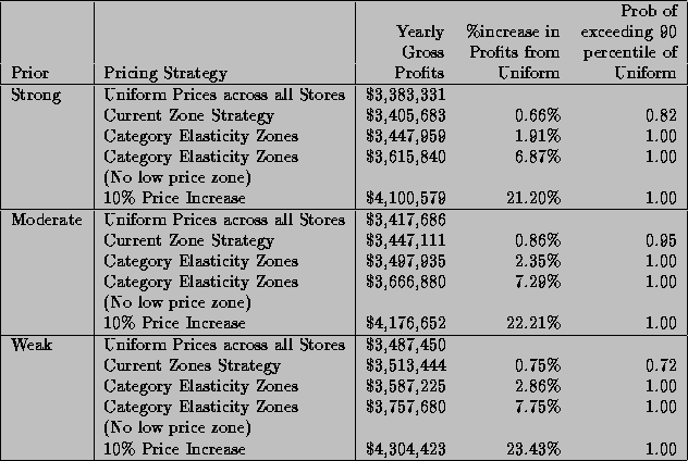
Table 7: Category Gross Profit Changes under various Pricing Strategies
To simplify our discussion about a store's price response, we develop an overall measure of the store's response to proportional price movements (i.e., the category elasticity). (See also Hoch et al. 1995.) The motivation of the category elasticity is to measure the effect on movement of a 1% increase (or decrease) of all the prices in the category. Our primary purpose is to construct a summary measure for labeling each store as price sensitive or insensitive. Formally the category elasticity is:

Where  is the total category movement,
 is the vector of movement market shares,
  is the cross
elasticity matrix evaluated at the average price for store s, and
 is a vector of ones.
To illustrate the dispersion of the category price elasticities using a moderate prior we plot each as a thermometer against its location in Figure 9. The thermometer's box shows the total range of the category elasticities (all boxes have the same height). The most price sensitive store is located on the South Side of Chicago with a category price elasticity of -1.87 (s.e.=.23). The least price sensitive store is in the northwest suburb of Arlington Heights, it has a category elasticity of .15 (s.e.=.12). (This is the only store that shows a positive category elasticity.) The shaded area within the box represents the posterior mean of the store's category elasticity. The average category elasticity across the stores is -.85 with a standard deviation of .31, three quarters of the stores have inelastic category price responses.
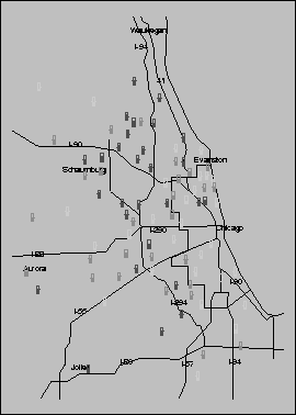
Figure 9: Category Price Elasticity
To ease the identification of stores we shade the thermometers. The most and least price sensitive third of the stores have the lightest and darkest shading respectively. The map allows us to observe that the largest geographic concentration of the price sensitive stores are located on the south side of Chicago, and the least price sensitive stores in the northwest suburbs. Notice that price sensitivities can change very quickly with price sensitive stores being located very closely to insensitive ones.
A natural question is whether the retailer's current assignment of stores to each pricing zone can be improved upon. To set up a better store-segmentation strategy the retailer could assign stores based upon their category-level elasticities. To keep the current zone strategy comparable with this new strategy we allocate the same number of stores to each price zone. The most inelastic stores are assigned to the high price zone, and the most elastic ones are assigned to the low price zone. These zones would increase expected profits to 2.35% over a uniform strategy. This improved zone scheme would result in a three-fold increase in profits that are now attributable to micro-marketing policies using Dominick's current zone strategy.
If we were to look at these results on a store by store basis we would see that stores with price increases have increased profits, and stores with price decreases have lower profits. This is the result of the low category price sensitivity of even our most price sensitive stores. Our improved zone classification scheme has increased the profitability of the high price zone, while the stores in the low price zone have been chosen to lessen the profit loss. Compared to this improved zone classification scheme, a better strategy is to simply discontinue the low price zone segment, or even better to simply increase the prices in all stores. If we combine the low and medium price zones under our category elasticity zones we would see a 7.29% increase in expected profits. Whereas if we simply raise the prices in all stores, we would realize a 22.21% increase. Notice that less than a quarter of the stores are in this high price zone, but total profits increase by more than a quarter. This disproportionate increase is the result of carefully selecting stores with the least price response.
This paper has shown that store-level differences in demand at the product can be measured. Furthermore these differences in price sensitivities translate into significant profit gains for the retailer. Beyond the question of statistical significance there is also the question of whether the magnitude of these profit increases are managerially significant. Our results indicate that micro-marketing strategies result in roughly a 3% increase in gross profits. Gross profits only consider the difference between the retail price and the retailer's cost, and do not reflect administrative and other selling costs. For refrigerated juices, gross profits are around 25%, which is the average for supermarket retailers (Supermarket Business 1992). On the otherhand operating profits were around 3% in 1993 (see publicly disclosed financial statements or a summary in Forbes 1994). If we assume that these micro-marketing increases are consistent across categories, then a 3% increase in gross profits would translate into a .75% increase in the retailer's operating profit margin or a 25% increase in operating profits.
It is difficult to know whether these results generalize to other retailers or whether these results are peculiar to this retailer at this specific time. But the supermarket retailer considered in this paper follows a Hi-Lo pricing strategy, which is the most commonly employed pricing strategy in this industry. Therefore we are optimistic that these results can be generalized to other retailers, in addition previous research suggests that these results will most likely generalize across categories (Hoch et al. 1995).
Our purpose has been to generate realistic estimates of the increases on profits given model and data limitations. To do this we have advocated placing constraints on promotion, revenue, and average price to guarantee there will be no change from current uniform pricing strategies. Our purpose has been to give a conservative estimate of the effects of micro-marketing pricing strategies. As these constraints are lifted off it becomes apparent that the retailer is systematically underpricing. While these predictions may seem disputable, they correlate well with results from studies conducted with the Micro-Marketing Project at the University of Chicago (Dreze, Hoch, and Purk 1993) which show a 10% increase in prices results in an 15% increase in profits averaged across 17 different categories. But clearly there is a need for future research to determine how cross-category substitution, loss leaders, and a store's image are affected on a long term basis.
A further reason to believe that these estimates on the profitability of micro-marketing strategies are conservative is that we have not exploited the retailer's dynamic cost structures (i.e., forward buying and promotional offers). We would expect that the retailer's costs would drop due to more efficient inventory allocation to each store. Furthermore previous research into promotions by Jeuland and Narasimhan (1985) advanced a price discrimination mechanism for promotions that would suggest that micro-marketing feature policies could be successful. If we were to allow feature prices to be store specific, we would expect a 7.72% increase in store profits instead of a 3.46% increase. Although this seems a promising direction, it is difficult to gauge consumer and competitive reaction. Therefore, we leave the specification of joint pricing and promotion micro-marketing strategies to future research.
The results presented in this paper show that the information contained in the retailer's store-level scanner data is an underutilized resource. By exploiting this information using newer and more powerful computational techniques retailers can better appreciate its value. There are profit incentives to the manager to better utilize the data resources that are available. The implication is that profits can be increased beyond what they are currently. This shows that gains can be made by using this information more efficiently. This also raises a question for a future research to study how limits on management's analytical capacities constrain a retailer's ability to use this information effectively.
The Gibbs sampler requires the solution of the conditional distributions, which can be easily derived due to the hierarchical structure of the model. For a good introduction to the Gibbs sampler see Casella and George (1992). The Gibbs sampler requires sequentially randomly sampling from each of the conditional distributions. It has been shown by Gelfand and Smith (1990) and Gelfand et al. (1990) that these draws converge in distribution to the posterior marginal distributions. The procedure is:
 sets of random numbers with each set
being drawn as:


Where  denotes x as a draw from the density
 , and k denotes the iteration.
 sets of draws to estimate the posterior
marginal distributions.
This means that the problem reduces to solving the conditional distributions of each parameter. These solutions are readily available due to the model's hierarchical structure and the affine nature of the normal and Wishart distributions (Anderson 1984, pp. 84 and 268-269). The solutions to the conditional distributions are:
 is a SUR model

 is drawn from an inverted wishart distribution

 is a multivariate regression

 is drawn from an inverted wishart distribution

These
conditional distributions are understood to also depend upon the prior
parameters and the data, and Z is a block diagonal matrix with
 on the diagonal.
The following parameters and data are
supplied by the analyst:

As an additional step in our procedure we also compute the conditional distribution of expected profits. Using the properties of the log-normal distribution we find:

For each store we will sum over all 52 weeks and iterations and divide by the number of iterations, this yields an estimate the marginal posterior profit distribution. Since these calculations are highly computer intensive when applying numerical optimization techniques we use every tenth Gibbs iteration, for a total of 110 iterations. This posterior is conditional only to the given pricing strategy. Therefore no bias is introduced in the profit function as is usually the case when the distribution of the parameter estimates is not accounted for (Blattberg and George 1992).
Stacking our individual store models from Chapter 3.2 we have:


Where the matrices without the store subscript denote the chain-wide information:

 is the identity matrix of dimension T. According to Smith
(1973) if
  and
and  and
and  are known
then we can show that the posterior distribution is:

where


and

With the LS-estimates defined in the usual way:

and


Allenby, G. (1989), ``A Unified Approach to Identifying, Estimating and Testing Demand Structures with Aggregate Scanner Data'', Marketing Science, 8, 265-280.
Allenby, G. and P. Rossi (1991b), ``Quality Perceptions and Asymmetric Switching Between Brands'', Marketing Science, 10, 185-204.
Anderson, T. W. (1984), An Introduction to Multivariate Statistical Analysis, New York: Wiley.
Bawa, K. and R. Shoemaker (1987), ``The Coupon-Prone Consumer: Some Findings Based on Purchase Behavior Across Product Classes'', Journal of Marketing 51, 99-110.
Bawa, K. and R. Shoemaker (1989), ``Analyzing Incremental Sales From a Direct Mail Coupon Promotion'', Journal of Marketing 53, 66-78.
Becker, G. (1965), ``A Theory of the Allocation of Time'', Economic Journal 75, 493-517.
Blattberg, R., T. Buesing, P. Peacock and S. Sen (1978), ``Identifying the Deal Prone Segment'', Journal of Marketing Research 15, 369-377.
Blattberg, R. and E. George (1991), ``Shrinkage Estimation of Price and Promotional Elasticities: Seemingly Unrelated Equations'', JASA 86, 304-315.
Blattberg, R. and E. George (1992), ``Estimation Under Profit-Driven Loss Functions'', Journal of Business and Economic Statistics, 10, 437-444.
Blattberg, R. and K. Wisniewski (1989), ``Price-Induced Patterns of Competition'', Marketing Science, 8, 291-309.
Casella, G. and E. George (1992), ``Explaining the Gibbs Sampler'', American Statistician 46, 167-174.
Deaton, A. and J. Muellbauer (1980), Economics and Consumer Behavior, Cambridge: Cambridge University Press.
Dickson, P. and A. Sawyer (1990), ``The Price Knowledge and Search of Supermarket Shoppers'', Journal of Marketing, 54, 42-53.
Dreze, X., S. Hoch, and M. Purk (1993), ``Data Driven Micro-Marketing: An Analysis of EDLP & Hi-Lo Pricing Strategies'', Working Paper, Micro-Marketing Research Project, University of Chicago.
Forbes, ``Annual Report on American Industry'', January 3, 1994.
Frank, R., W. Massy, and Y. Wind (1972), Market Segmentation, Prentice-Hall.
Gelfand, A., S. Hills, A. Racine-Poon, and A. Smith (1990), ``Illustration of Bayesian Inference in Normal Data Models Using Gibbs Sampling'', JASA 85, 972-985.
Gelfand, A. and A. Smith (1990), ``Sampling-Based Approaches to Calculating Marginal Densities'', JASA 85, 398-409.
Hoch, S., B. Kim, A. Montgomery, and P. Rossi (1995), ``Determinants of Store-Level Price Elasticity'', Journal of Marketing Research, 32, 17-29.
Jeuland, A. and C. Narasimhan (1985), ``Dealing-Temporary Price Cuts-by Seller as a Buyer Discrimination Mechanism'', Journal of Business, 58, 295-308.
Kamakura, W. and G. Russell (1989), ``A Probabilistic Choice Model for Market Segmentation and Elasticity Structure'', Journal of Marketing Research 26, 379-90.
Kumar, V. and R. Leone (1988), ``Measuring the Effect of Retail Store Promotions on Brand and Store Substitution'', Journal of Marketing Research 25, 178-85.
Lewbel, A. (1985), ``A Unified Approach to Incorporating Demographic or Other Effects into Demand Systems'', Review of Economic Studies, 20, 1-18.
Lindley, D. and A. Smith (1972), ``Bayes Estimates for the Linear Model'', Journal of the Royal Statistical Society, Series B, 34, 1-41.
Montgomery, A. (1994), ``The Impact of Micro-Marketing on Pricing Strategies'', Unpublished dissertation, Graduate School of Business, University of Chicago.
Montgomery, D. (1971), ``Consumer Characteristics Associated with Dealing: An Empirical Example'', Journal of Marketing Research 8, 118-20.
Rossi, P., R. McCulloch, and G. Allenby (1994), ``Hierarchical Modelling of Consumer Heterogeneity: An Application to Target Marketing'', Working Paper, University of Chicago.
Smith, A. (1973), ``A General Bayesian Linear Model'', Journal of the Royal Statistical Society, Series B, 35, 67-75.
Supermarket Business, September 1992.
Walters, R. (1991), ``Assessing the Impact of Retailer Price Promotions on Product Substitution, Complementary Purchase, and Interstore Sales Displacement'', Journal of Marketing 55, 17-28.
Walters, R. and S. MacKenzie (1988), ``A Structural Equations Analysis of the Impact of Price Promotions on Store Performance'', Journal of Marketing Research, 25, 51-63.
Webster, F. (1965), ``The 'Deal-Prone' Consumer'', Journal of Marketing Research 2, 186-9.
Zellner, A. (1971), An Introduction to Bayesian Inference in Econometrics, New York: Wiley.
This document was generated using the LaTeX2HTML translator Version 95 (Thu Jan 19 1995) Copyright © 1993, 1994, Nikos Drakos, Computer Based Learning Unit, University of Leeds.
The command line arguments were:
latex2html -split 0 newmorework.tex.
The translation was initiated by Heidi Rhodes on Tue Aug 6 15:54:47 EDT 1996