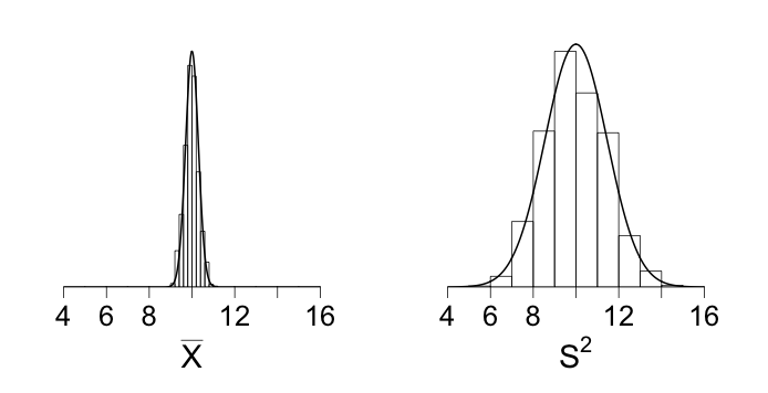
#  Script runs 1,000 simulations drawing a sample of size 100 from a
#  Poisson distribution, and then plots histograms of the estimated
#  means and estimated variances.
#
#  Figure caption: Histograms displaying distributions of X-bar and S
#  squared based on 1,000 randomly generated samples of size n = 100
#  froma Poisson distribution with mean parameter mu = 10.  In these
#  repeated samples, both X-bat and S squared have distributions that
#  are approximately normal.  Both distributions are centered at 10
#  (both estimators are unbiased) but the values of S squared
#  fluctuate much more than do the values of X-bar.


nSimulations <- 1000
nSamples     <- 100
lambda       <- 10

#  Generate all samples at once.
simulationSamples <- rpois( nSimulations * nSamples, lambda)
dim(simulationSamples) <- c( nSamples, nSimulations )

#  Now that we have a matrix of poisson samples, with 1000 columns and
#  100 rows, each column can be considered a simulation.
sampleMeans <- apply(simulationSamples, 2, mean)
sampleVariances <- apply(simulationSamples, 2, var)


xValues<-seq(4, 16, by = 0.01)

par(mfrow = c(1, 2))
par(xaxs = "i")
par(yaxs = "i")
par(mar = c(5, 3, 1, 3))

#  Plot the sample means histogram.
hist(sampleMeans, freq = FALSE,
     xlim = c(4, 16), ylim = c(0, 1.5),
     yaxt = "n", main = "", xlab = expression(bar(X)), ylab = "",
     cex.lab = 1.8, cex.axis = 1.6)

#  Add a line for the theoretical pdf of the sample mean.
#  This is normal with mean lambda and variance
sampleMeansVariance = lambda / nSamples
lines(xValues, dnorm(xValues, lambda, sqrt(sampleMeansVariance)), lwd = 2)

#  Plot the sample variances histogram.
hist(sampleVariances, freq = FALSE,
     xlim = c(4, 16), ylim = c(0, 0.3),
     yaxt = "n", main = "", xlab = expression(S^{2}), ylab = "",
     cex.lab = 1.8, cex.axis = 1.6)

#  Compute the variance of the sample variances and plot the
#  theoretical density.
sampleVariancesVariance <- (lambda/nSamples) + 2 * (lambda^2 / (nSamples - 1))
theoreticalPdf <- dnorm(xValues, lambda, sqrt(sampleVariancesVariance))
lines(xValues, theoreticalPdf, lwd = 2)

#  Print the figure as a postscript.
dev.print(device = postscript, "8.2.eps", horizontal = TRUE)

