# Plots autoregression coefficient estimates, the autocorrelation
# function, and the partial autocorrelation function for an
# autoregressive model on the residuals of a temperature model fit in
# other temp.R files.
#
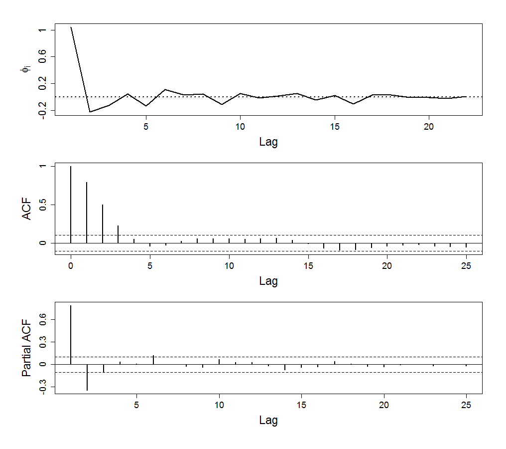
# Figure caption: Autoregressive model of order p = 22 for core
# temperature residuals. TOP: Coefficients theta-hat-i as a function
# of lag i. MIDDLE: the sample autocorrelation function. BOTTOM:
# The sample partial autocorrelation function.
# The Haell Miscellaneous library contains a variety of utility
# functions for statistical analysis, data manipulation, and LaTeX
# expressions.
library(Hmisc)
# First read in the temperature data, and assign column names.
temperatureDF <- read.table("data/temp.dat", col.names = c("Temp", "Time"))
temperature <- temperatureDF$Temp
time <- temperatureDF$Time
# We now want to regress our data against sinusoids with a period of 72.
# First create the sinusoids.
cosine <- cos(2 * pi * time/72)
sine <- sin(2 * pi * time/72)
# Then fit a linear model.
lm.temperature <- lm(temperature ~ cosine + sine)
temperatureResiduals <- lm.temperature$residuals
orderP <- 22
n <- 330
x <- array(0, dim = c(n, orderP))
range <- (orderP + 1):(orderP + n)
y <- temperatureResiduals[range]
for(i in 1:22) {
x[ , i] <- Lag(temperatureResiduals, i)[range]
}
# Fit autoregressive model without intercept.
ar.reg=lm(y ~ x - 1)
summary(ar.reg) # Display summary.
# Set graphical parameters.
par(oma = rep(2, 4))
par(mar = c(5, 5, 1, 1))
par(mfrow=c(3,1))
axis.size <- 1.4
label.size <- 1.8
# Plot estimated autocorrelation coefficients.
plot(1:22, ar.reg$coef, type="l",
xlab = "Lag", ylab = expression(phi[i]),
lwd=2, cex.lab = label.size, cex.axis = axis.size, yaxt = "n")
abline(h = 0, lty = 3, lwd = 2)
axis(2, at = seq(from = -0.2, to = 1, by = 0.4),
labels = seq(from = -0.2, to = 1, by = 0.4), cex.axis = 1.5)
# Plot sample autocorrelation function.
acf(temperatureResiduals, main = "",
cex.lab = label.size, cex.axis = axis.size,
lwd = 2, yaxt = "n", ci.col = 1)
axis(2, at = seq(from = 0, to = 1, by = 0.5),
labels = seq(from = 0, to = 1, by = 0.5), cex.axis = axis.size)
# Plot sample partial autocorrelation function.
pacf(temperatureResiduals, main = "",
cex.lab = label.size, cex.axis = axis.size,
lwd = 2, yaxt = "n", ci.col = 1)
axis(2, at = seq(from = -0.3, to = 0.6, by = 0.3),
labels = seq(from = -0.3, to = 0.6, by = 0.3), cex.axis = axis.size)
dev.print(device = postscript, "18.7.eps", horizontal = TRUE)