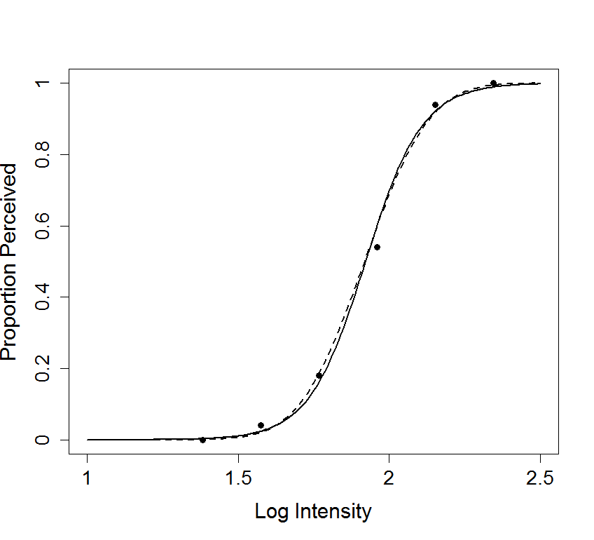
#  Figure 14.1 - Plots actual data, a logistic regression, and a
#  probit regression, in order to show that (a) the fits are good, and
#  (b) the logistic and probit models are very similar.
#
#  Figure caption: Two curves fitted to the data in Figure 8.9.  The
#  fitted curve from probit regression (dashed line) is shown together
#  with the fitted curve from logistic regression.  The fits are very
#  close to eachother.


#  MPDiR loads the HSP data set.  The data are from Hecht et al, and
#  show, in 50 trials, whether or not light flashes of a certain log10
#  intensity were observed by a subject.
#  
library(MPDiR)

chosenRun     <- "R1"    #  Use Run 1.
chosenSubject <- "SS"    #  Choose the subject S.S.
chosenData    <- HSP$Run == chosenRun & HSP&Obs == chosenSubject
dataForOneRun <- HSP[chosenData, ]

#  Pull the data for one run.  
lightIntensiy   <- log10(dataForOneRun$Q)
percentDetected <- dataForOneRun$p / 100  #  Scale percentages to (0,1).

#  Fit logistic and probit models.  
modelEquation <- percentDetected ~ lightIntensity
logisticModel <- glm(modelEquation, family = binomial(link = "logit"))
probitModel   <- glm(modelEquation, family = binomial(link = "probit"))


lightValues <- data.frame( x = seq(from = 1, to = 2.5, by = 0.01))



#  Plot actual points and the models' fits.
plot(lightIntensity, percentDetected)
     xlim = c(1, 2.5), ylim = c(0, 1),
     xlab = "Log Intensity", ylab = "Proportion Perceived", main = "",
     xaxt = "n", yaxt = "n", pch = 16, cex.lab = 1.5)


lines(lightValues, predict(logisticModel, newdata = lightValues),
      lty = 1, lwd = 2)
lines(lightValues, predict(probitModel, newdata = lightValues),
      lty = 2, lwd = 2)


axis(1, at = seq(from = 1, to = 2.5, by = 0.5), cex.axis = 1.4)
axis(2, at = seq(from = 0, to = 1, by = 0.2), cex.axis = 1.4)

#legend("topleft", c("Logistic", "Probit"), lty = c(1, 2),
#              lwd = c(2, 2), cex = 1.5)

dev.print(device = postscript, "14.1.eps", horizontal = TRUE)