#  Figure 10.3
#
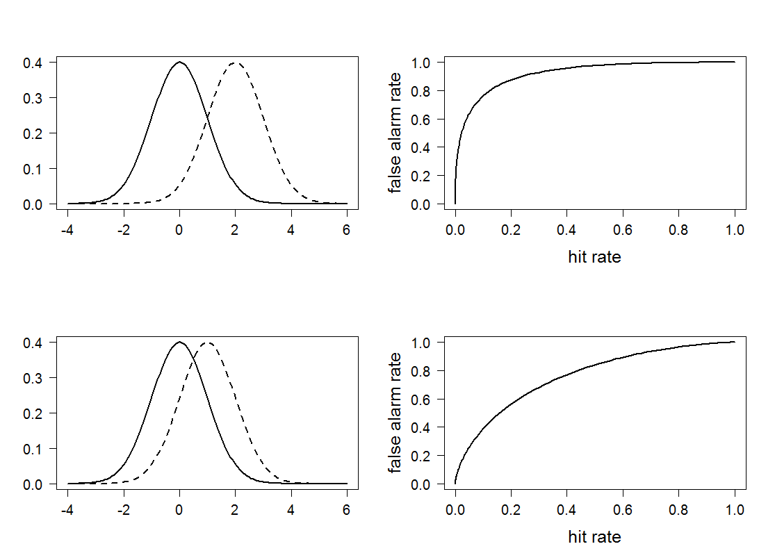
#  Figure caption: Two pairs of normal distributions and the
#  resulting ROC curves.  The left hand side shows the pair of pdfs
#  for N(0,1) (solid) and N(delta, 1) (dashed) and to the Right are
#  the corresponding ROC curves.
#
#  Top delta = 2.  Bottom delta = 1.

#  Initialize a postscript object and set some figure parameters.  
postscript("roc.ps")
par(cex.lab = 1.5)
par(cex.axis = 1.25)
par(las = 1)
par(mfrow = c(2, 2) )

#  Initialize distribution parameters.
x <- seq(-4, 6, length = 200)
deltas = c(2, 1)

#  Do plots for both deltas in a loop. 
for (i in 1:2) {
    delta <- deltas[1]
    matplot(x, cbind(dnorm(x, 0, 1), dnorm(x, delta, 1)),
            type = "l",xlab = "", ylab = "", col  =  1, lwd  =  2)

    plot(1 - pnorm(x, 0, 1), 1 - pnorm(x, delta, 1),
         type = "l", xlab = "hit rate", ylab = "false alarm rate", lwd  =  2)
    }

dev.off()