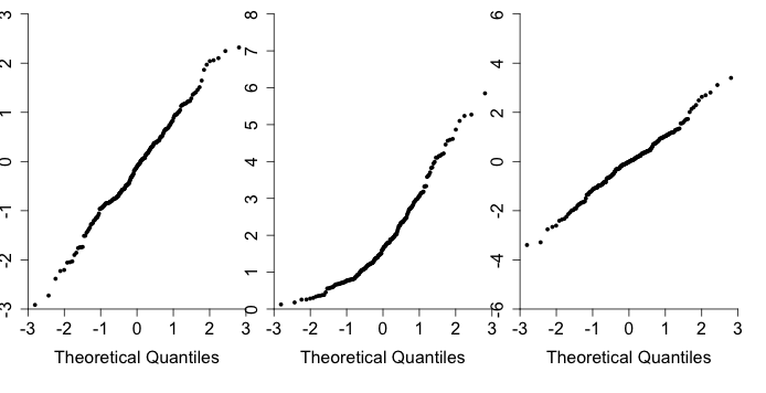
#  This script plots three QQ-normal plots, for a normal, gamma, and t
#  distribution.

#  Set up the graphics device.
par(mfrow = c(1, 3))
par(xaxs = "i")
par(yaxs = "i")

#  Set some graphical parameters.
standard.axis <- seq(from = -3, to = 3, by = 1)
y.axis <- seq(from = -3, to = 3, by = 1)
axis.size <- 1.5
point.type <- 16
label.size <- 1.5
size <- 0.8

#  Set some simulation parameters.
N = 200

#  Plot the QQ normal plot for an actual normal sample.
qqnorm(rnorm(N), xlim = c(-3, 3), ylim = c(-3, 3),
       main = "", ylab = "", xaxt = "n", yaxt = "n", bty = "n",
       cex.lab = label.size, pch = point.type, cex = size)
axis(1, at = standard.axis, labels = standard.axis, cex.axis = axis.size)
axis(2, at = standard.axis, labels = standard.axis, cex.axis = axis.size)

#  Plot the QQ normal plot for a gamma sample.
qqnorm(rgamma(N, 2.5, 1.25), xlim = c(-3, 3), ylim = c(0, 8),
       main = "", ylab = "", xaxt = "n", yaxt = "n", bty = "n",
       cex.lab = label.size, pch = point.type, cex = size)
axis(1, at = standard.axis, labels = standard.axis, cex.axis = axis.size)
gamma.y.axis <- seq(from = 0, to = 8, by = 1)
axis(2, at = gamma.y.axis, labels = gamma.y.axis, cex.axis = axis.size)

#  Plot the QQ normal plot for a t sample.
qqnorm(rt(N, 4), xlim = c(-3, 3), ylim = c(-6, 6),
       main = "", ylab = "", xaxt = "n", yaxt = "n", bty = "n",
       cex.lab = label.size, pch = point.type, cex = size)
axis(1, at = standard.axis, labels = standard.axis, cex.axis = axis.size)
t.y.axis <- seq(from = -6, to = 6, by = 2)
axis(2, at = t.y.axis, labels = t.y.axis, cex.axis = axis.size)

#  This seems as though it is figure 3.10, but things may have changed
#  from the May 15th version.
dev.print(device = postscript, "3.11.eps", horizontal = TRUE)

