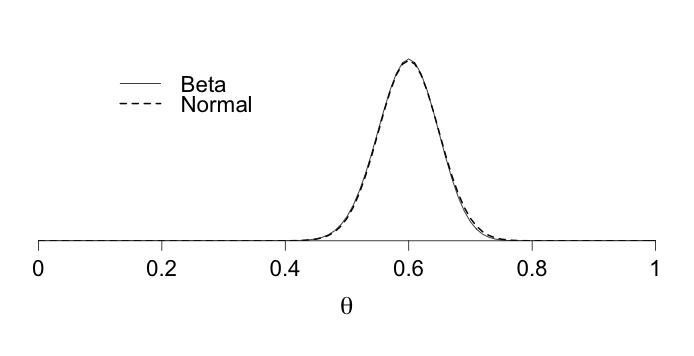
#  This script shows a very close Normal approximation for a Beta distribution.

#  Set up the graphics device.  
par(yaxs = "i")
par(mar = c(5, 1, 0, 1))

#  Set some graphical parameters.
label.size <- 1.6

#  Start with an empty plot, setting up the window.
plot(0, 0, xlim = c(0, 1), ylim = c(0, 10), type = "n", 
     main = "", xlab = expression(theta), ylab = "", 
     xaxt = "n", yaxt = "n", bty = "n", cex.lab = label.size)

#  Plot both densities. 
x.values <- seq(from = 0, to = 1, by = 0.01)
lines(x.values, dbeta(x.values, 61, 41), lty = 1, lwd = 1)
lines(x.values, dnorm(x.values, .6, 0.049), lty = 2, lwd = 2)

#  Clean up the axes.  
x.axis <- seq(from = 0, to = 1, by = 0.2)
axis(1, at = x.axis, labels = x.axis, cex.axis = 1.4)

#  Add a legend.
legend(0.1, 8, c("Beta", "Normal"), lty = c(1, 2), 
       bty = "n", cex = 1.4, lwd = c(1, 2))

dev.print(device = postscript, "8.8.eps", horizontal = TRUE)