#  Creates two histograms, one of them log-scale, for the saccadic
#  reaction time data from figure 2.1
#
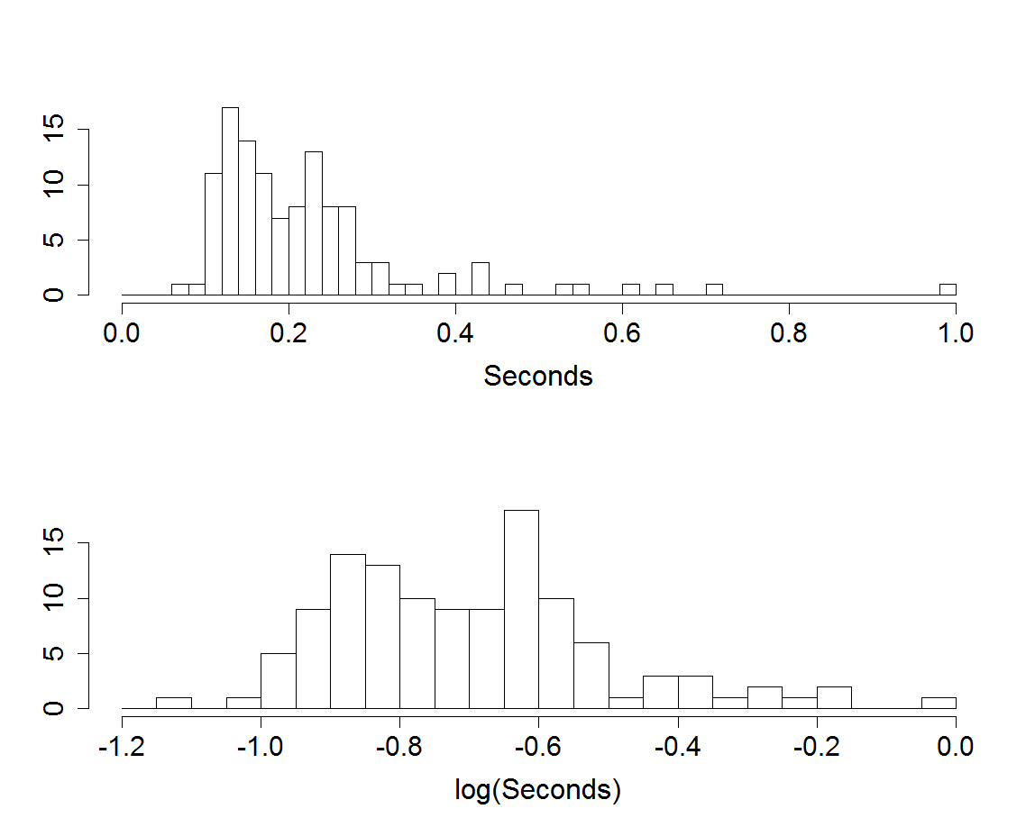
#  Figure caption:  Histograms of eye saccade data.  Top display is
#  for data in the original scale, bottom display is for the same
#  data after being transformed by log10.  The data are distributed
#  more symmetrically in the log scale.  

patient1 <- read.table("data/p3359b.csv")[[1]]
log_patient1 <- log10(patient1)

dev.new(width = 10, height = 8)
par(mfrow = c(2, 1))
pat(oma = c(2, 2, 0, 0))

#  Histogram in original scale.  

hist(patient1, breaks = seq(from = 0, to = 1, by = 0.02), xlab = "Seconds", ylab = "", main = "", yaxt = "n", ylim = c(0, 18), cex.lab = 1.6, cex.axis = 1.5)
axis(2, at = seq(from = 0, to = 15, by = 5), labels = seq(from = 0, to = 15, by = 5), cex.axis = 1.5)

#  Histogram in log scale.  

hist(log_patient1, seq(from = -1.2, to = 0, by = 0.05), xlab = "log(Seconds)", ylab = "", main = "", yaxt = "n", ylim = c(0, 18), cex.lab = 1.6, cex.axis = 1.5)
axis(2, at = seq(from = 0, to = 15, by = 5), labels = seq(from = 0, to = 15, by = 5), cex.axis = 1.5)