#  This script plots a binomial likelihood function as a function of x,
#  and as a function of theta for fixed x.  
#
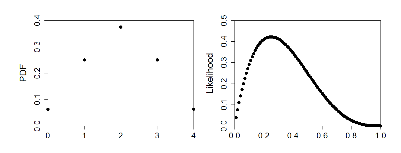
#  Figure caption:  Comparison of pdf of f(x|theta) when viewed as
#  a function of x with theta fixed at 0.5 (on left) or of theta
#  with x fixed at x = 1 (on right).  On the right hand side, the
#  pdf is evaluated for 99 equally spaced values of theta from 0.01
#  to 0.99.  


#  Set graphical device parameters.  
par(mfrow = c(1, 2))
par(xaxs = "i")              #  Enables exact specification of plot window.
par(yaxs = "i")
par(oma = rep(2, 4))
par(mar = c(2, 5, 1, 1))
par(xpd = TRUE)             #  Plotting clipped to figure region, rather than 
                            #  plot region.  

#  Set some plotting parameters.
point.type <- 16 
point.size <- 1.2
label.size <- 1.6
axis.size <- 1.4

#  Plot the density evaluated for several possible x values.
x.values <- seq(from = 0, to = 4, by = 1)
plot(x.values, dbinom(x.values, size = 4, prob = 0.5), 
     xlim = c(0, 4), ylim = c(0, 0.4), pch = point.type, cex = point.size, 
     main = "", xlab = "X", ylab = "PDF", cex.lab = label.size, cex.axis = axis.size)

#  Plot the density as a function of theta.
theta.values <- seq(from = 0.01, to = 1, by = 0.01)
plot(theta.values, dbinom(x = 1, size = 4, prob = theta.values), 
    xlim = c(0, 1), ylim = c(0, 0.5), pch = point.type, cex = point.size, 
    main = "", xlab = expression(theta), ylab = "Likelihood", cex.lab = label.size, cex.axis = axis.size)

#  Close the graphics device.  
dev.print(device = postscript, "7.2.eps", horizontal = TRUE)