# Code initially written by Rob Kass, Revised by Patrick Foley.

#  First read in the temperature data, and assign column names.
temperatureDF <- read.table("data/temp.txt", col.names = c("Temp", "Time"))
temperature <- temperatureDF$Temp
time <- temperatureDF$Time

#  We now want to regress our data against sinusoids with a period of 72.
#  First create the sinusoids.
cosine <- cos(2 * pi * time/72)
sine <- sin(2 * pi * time/72)

#  Then fit a linear model.
lm.temperature <- lm(temperature ~ cosine + sine)


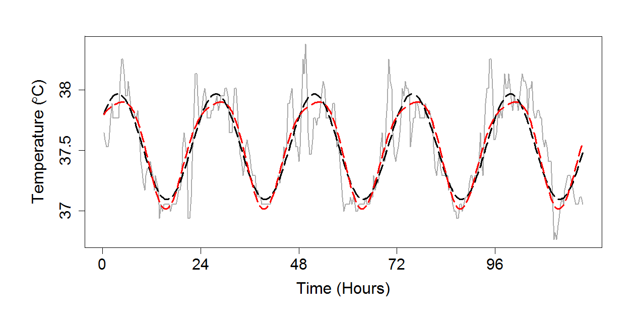
# Now set up the jpeg for figure 18.2, which shows the raw temperature
# data as well as a single frequency model.
jpeg("figure18.2.jpg")

#  Now we create the model in figure 18.3, which includes a term at
#  twice the fundamental frequency.
cosine2 <- cos(2 * pi * time * 2/72)
sine2 <- sin(2 * pi * time * 2/72)

#  And again, we fit the linear model.
twoFrequencyModel <- lm(temperature ~ sine + cosine + cosine2 + sine2)

#  Then set up the jpeg device and plot the raw data.
par(oma = rep(2, 4))
par(mar = c(4, 5, 1, 1))

plot(time, temperature, type = "l", xaxt = "n", yaxt = "n", xlab = "Time (Hours)", ylab = expression(paste("Temperature (",degree,"C)")), main = "", cex.lab = 1.6, lwd = 2, col = "darkgrey")

#  Add the two models' fits, as two different line types, and
#  close the device.
lines(time, lm.temperature$fit, lwd = 3, lty = 5)
lines(time, twoFrequencyModel$fit, lwd = 3, col = 2, lty = 5)
axis(1, at = seq(from = 0, to = 288, by = 72), labels = seq(from = 0, to = 96, by = 24), cex.axis = 1.5)
axis(2, at = seq(from = 36.5, to = 38.5, by = 0.5), labels = seq(from = 36.5, to = 38.5, by = 0.5), cex.axis = 1.5)

dev.off()

