# This figure shows empirical CDFs for a small and a large sample
# from the gamma distribution to demonstrate their convergence to
# the empirical CDF.
#
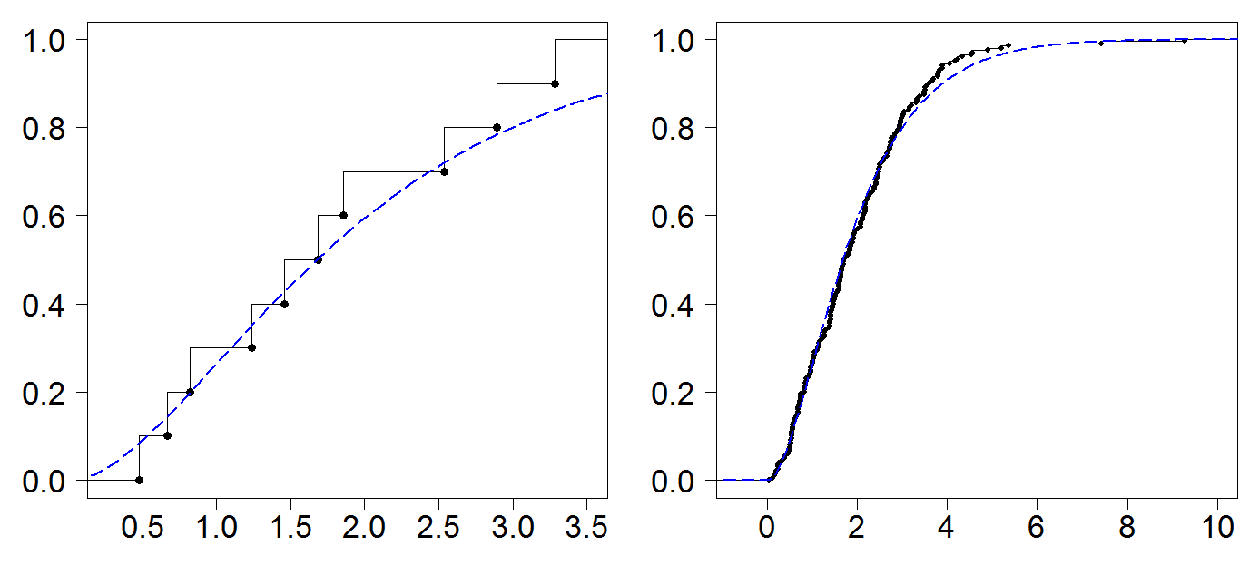
#  Figure caption:  Convergence of the empirical cdf to the
#  theoretical cdf.  The left panel displays the empirical cdf for
#  a random sample of size 10 from the gamma distribution whose pdf
#  is the top right band panel of figure 3.3, together with the
#  gamma cdf.  The right panel shows the empirical cdf for a random
#  sample of size 200, again with the gamma cdf.  In the right
#  panel, the empirical cdf is quite close to the theoretical gamma
#  cdf.

#  Set graphical parameters 
postscript("ecdf.ps")
par(cex.lab=2)
par(cex.axis=1.75)
par(las=1)
par(mfrow=c(1,2))
par(mar = c(4, 4, 1, 1))

#  Generate data for samples of sizes 10 and 200.
smallSample = rgamma(10, 2)
largeSample = rgamma(200, 2)

#  Plot the smaller sample's empirical CDF, and add a line for the
#  theoretical CDF.
xvals = sort(smallSample)
yvals = (0:10)/10
fhat = stepfun(xvals, yvals, right = TRUE)
plot(fhat, xlab = "", ylab = "", main = "", pch = 16, cex = 1)
xseq = seq(-1, 12, length = 300)
lines(xseq, pgamma(xseq, 2), lty = 5, lwd = 2, col = 4)

#  Do the same for the larger sample.
xvals = sort(largeSample)
yvals = (0:200)/200
fhat = stepfun(xvals, yvals, right = TRUE)
plot(fhat, xlab = "", ylab = "", main = "", pch = 16, cex = 0.7)
xseq = seq(-1, 12, length = 300)
lines(xseq, pgamma(xseq, 2), lty = 5, lwd = 2, col = 4)

#  Close the graphics device.
dev.off()
#try library(Hmisc); use ecdf