#  Plots the binomial density for four different values of N.

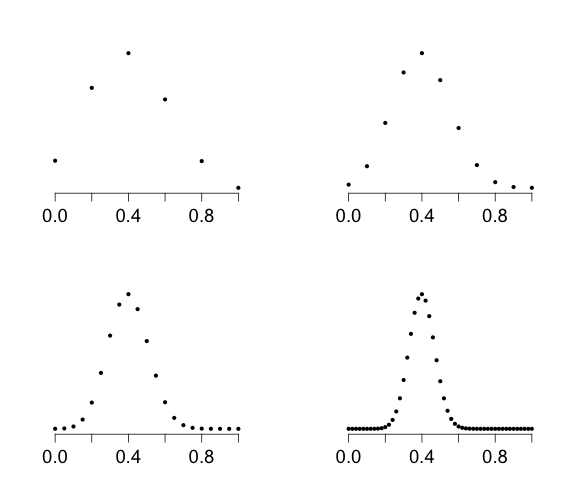
#  Figure caption: The pdf of the binomial mean X-bar when p = 0.4
#  for four different values of n.  As n increases, the
#  distribution becomes concentrated (the standard deviation of the
#  sample mean becomes small), with the center of the distribution
#  getting close to muX = 0.4 (the LLN).  In addition, the
#  distribution becomes approximately normal (the CLT).  

#  Set up the graphics device.
par(mfrow = c(2, 2))
par(mar = rep(3, 4))

#  Set up the binomial parameters.
p <- 0.4
n.values <- c(5, 10, 20, 50)


for (i in 1:4) {

    n <- n.values[i]
    x.values <- 0:n
    means <- x.values / n

    plot(means, dbinom(x.values, n, p)
         xlim = c(0,1),
         main = "", xlab = "", ylab = "", 
         xaxt = "n", yaxt = "n", bty = "n", pch = 16, cex = 0.7)
    axis(1, at = seq(from = 0, to = 1, by = 0.2), cex.axis = 1.4)
    
}


dev.print(device = postscript, "6.1.png", horizontal = TRUE)