# Set up the graphics device.
par(mfrow = c(1, 2))
par(mar = c(5, 3, 1, 2))
# Set up some parameters for both time series.
n.points <- 100
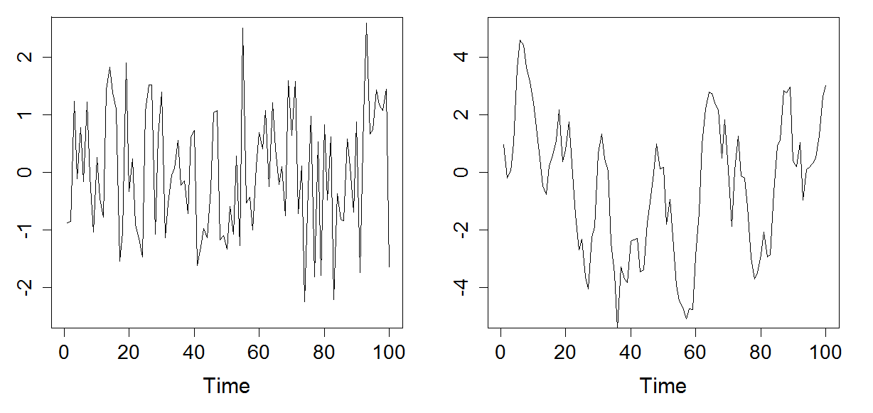
# Plot an AR-0 time series.
plot(1:n.points, rnorm(n.points), type = "l",
xlim = c(0, n.points), ylim = c(-2.5, 2.5),
xaxt = "n", yaxt = "n", main = "", xlab = "Time", ylab = "",
cex.lab = 1.5)
# Clean up axes.
x.axis <- seq(from = 0, to = n.points, by = 20)
y.axis <- seq(from = -3, to = 3, by = 1)
axis.size <- 1.4
axis(1, at = x.axis, labels = x.axis, cex.axis = axis.size)
axis(2, at = y.axis, labels = y.axis, cex.axis = axis.size)
# Simulate an autoregressive time series.
time.series <- arima.sim(model = list(ar = c(.9)), n = n.points)
# Plot the AR series.
plot(1:n.points, time.series, type = "l",
xlim = c(0, n.points), ylim = c(-5, 5),
xaxt = "n", yaxt = "n", main = "", xlab = "Time", ylab = "",
cex.lab = 1.5)
# Clean up axes again, but change the y-axis.
y.axis <- seq(from = -4, to = 4, by = 2)
axis(1, at = x.axis, labels = x.axis, cex.axis = axis.size)
axis(2, at = y.axis, labels = y.axis, cex.axis = 1.4)
dev.print(device = postscript, "12.7.eps", horizontal = TRUE)