%  Creates two histograms, one of them log-scale, for the saccadic
%  reaction time data from figure 2.1
%
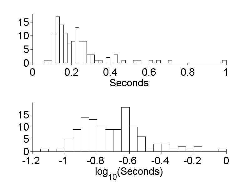
%  Figure caption:  Histograms of eye saccade data.  Top display is
%  for data in the original scale, bottom display is for the same
%  data after being transformed by log10.  The data are distributed
%  more symmetrically in the log scale.  

patient1 = csvread('p3359b.csv', 0, 0);
log_patient1 = log10(patient1);


%  Histogram in original scale.  
subplot(2, 1, 1)
hist(patient1, 0.01:0.02:0.99)
set(gca,'Box','off', 'FontSize', 20, ...
        'XLim', [0, 1], 'YLim', [0, 18], ...
        'XTick', 0:0.2:1, 'YTick', 0:5:15, 'TickDir', 'out')

spikehist = findobj(gca, 'Type', 'patch');
set(spikehist, 'FaceColor', 'w')
xlabel({'Seconds'}, 'FontSize', 20)


%  Histogram in log scale.  
subplot(2, 1, 2)
hist(log_patient1, -1.175:0.05:-0.025)
set(gca,'Box','off', 'FontSize', 20, ...
        'XLim', [-1.2, 0], 'YLim', [0, 20], ...
        'XTick', -1.2:0.2:0, 'YTick', 0:5:15, 'TickDir', 'out')

spikehist = findobj(gca, 'Type', 'patch');
set(spikehist, 'FaceColor', 'w')
xlabel({'log_{10}(Seconds)'}, 'FontSize', 20)


%  Set the position of the figure.  
set(gcf, 'Position', [200, 100, 800, 600])