Regression

The file geyser.dat contains data about Old Faithful Geyser, a popular tourist attraction. A geologist was interested in predicting the length of time between eruptions based on the duration of eruptions. He observed the geyser several times in August 1978, and several more times in August 1979.

> geyser <- read.table("geyser.dat",col.names=c("date","interval","duration","is.aug.78","is.aug.79"))
> attach(geyser)

The data file consists of what day the observation took place, the interval between eruptions (in minutes), the duration of the preceding eruption (in minutes), a 0/1 indicator variable for August 1978, and another 0/1 indicator variable for August 1979.

> motif()
> plot(duration, interval)

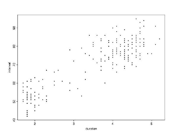
This picture shows an upward sloping relationship between duration and interval. The longer the eruption, the more time until the next eruption.

Let's start with only one predictor, duration. The formula would be ``interval modeled by duration'', which is interval ~ duration . The function to create a regression model is lm, for Linear Model.

> lm(interval ~ duration)
Call:
lm(formula = interval ~ duration)

Coefficients:
 (Intercept) duration
    33.90084 10.37363

Degrees of freedom: 221 total; 219 residual
Residual standard error: 6.170498

The lm function creates an object of class ``linear model'', and returns its value. The value includes the coefficients and other information. It is a good idea to store this object someplace so that you can update it and refer to it as you proceed with the analysis.

> geyser.lm <- lm(interval ~ duration)

The summary function, which you have probably used to generate summary statistics about a vector, comes in handy with model objects.

> summary(geyser.lm)

Call: lm(formula = interval ~ duration)
Residuals:
   Min     1Q  Median    3Q   Max
 -14.1 -4.507 -0.4701 4.194 16.83

Coefficients:
              Value Std. Error t value Pr(>|t|)
(Intercept) 33.9008  1.4409    23.5277  0.0000
   duration 10.3736  0.3850    26.9428  0.0000

Residual standard error: 6.17 on 219 degrees of freedom
Multiple R-Squared: 0.7682
F-statistic: 725.9 on 1 and 219 degrees of freedom, the p-value is 0

Correlation of Coefficients:
         (Intercept)
duration -0.9576

The summary command provides a bevy of useful information, including p-values, multiple R-Squared, and correlation. Based on this information, it looks like duration is a very good predictor of interval .

Another way to examine regression output is graphically, using the plot command. When given regression output as its argument, plot will produce six diagnostic plots. To see them all, you must split the plotting window into six or more parts. For instance, make it into a 2 by 3 grid of windows.

> par(mfrow=c(2,3))
> plot(geyser.lm)

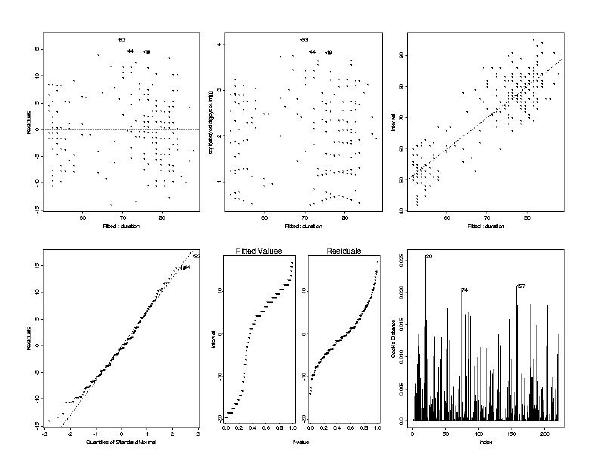
The par(mfrow=c(2,3)) command divided the graphics window into six separate windows. To change it back to normal, do par(mfrow=c(1,1)) (that is, one row by one column). This command will take effect when the next plot is executed.

The six plots show useful diagnostic information, such as plots of residuals vs. fitted values, a quantile-normal plot, and a Cook's distance plot (the influence of each data point on the final model, large values indicate high influence).

Other functions which can be used on model objects include residuals (returns a vector of the residuals) and fitted (returns a vector of the fitted values).