A Statistical Example with Data Frames

Ohio State University did an experiment comparing air-filled and helium-footballs. A novice punter kicked each football 39 times (alternating between the air-filled and the helium-filled ball) and the experiment recorded the distance (in yards) travelled by each ball. These data are in the file football.dat. Read that file into a data frame and attach to it.

Next open a graphics window by typing motif() or x11() on a UNIX machine or win.start() on a Windows machine.

A good place to start might be with summary statistics for helium footballs and regular footballs.

> summary(Helium)
 Min. 1st Qu. Median  Mean 3rd Qu. Max.
   11    24.5     28 26.38      30   39
> summary(Air)
 Min. 1st Qu. Median  Mean 3rd Qu. Max.
   15    23.5     26 25.92    28.5   35

It looks like the helium footballs go a little further on average. Next we could look at box plots:

> boxplot(Helium, Air)

Note that when you do this, S-PLUS does not label anything. We can add some titles:

> title(ylab="Distance Traveled")
> title(xlab="Helium (left) vs. Air (right)")
> title("Boxplots by Football Type")

The box plot for helium-footballs shows a few outliers. Were these from when the kicker was beginning to kick the footballs and hadn't learned to kick them far yet, or were they accidental mis-kicks from later in the experiment? We can plot the helium distances in order and see what they show.

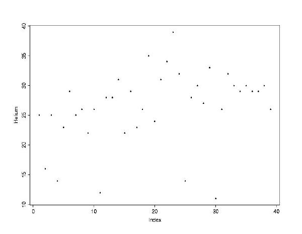
> plot(Helium)

This plot shows that there were a couple of relatively short kicks at the beginning, and then three shorts ones later which look to be outliers.

S-PLUS has a function which allows you to select points on a graph by using the mouse. Once you have plotted a graph, you can run identify on that graph. This allows you to identify the index of a point by clicking with the left mouse button and to stop identifying by clicking with the center mouse button (this is with a three-button mouse; if you have fewer buttons, play around and figure out how to use identify using your mouse). I typed identify(Helium) and clicked on each of the three points to get their index number.

The three outliers are observations number 11, 25, and 30. Now consider the distance the other helium footballs travelled:

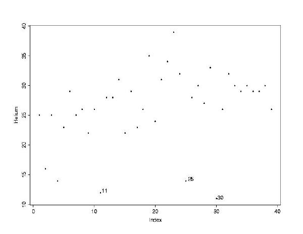
> summary(Helium[-c(11,25,30)])
 Min. 1st Qu. Median  Mean 3rd Qu. Max.
   14      25     28 27.56      30   39

The median was unaffected by removing those three observations, but the mean increased slightly. It looks like helium-filled footballs travel about 1.6 yards further than regular footballs. The way to test whether this is significant is with a paired t-test (that is, the first air-kick compared to the first helium-kick, the second air-kick compared to the second helium-kick, etc. ). We must exclude the 11th, 25th and 30th distances travelled by air-filled footballs in order to have matched pairs for all footballs.

> t.test(Helium[-c(11,25,30)],Air[-c(11,25,30)], paired=T)

         Paired t-Test

data:  Helium[ - c(11, 25, 30)] and Air[ - c(11, 25, 30)]
t = 1.4923, df = 35, p-value = 0.1446
alternative hypothesis: true mean of differences is not equal to 0
95 percent confidence interval:
 -0.5405538  3.5405538
sample estimates:
 mean of x - y
           1.5

The p-value is .14, so it appears that there is no significant difference in the distance travelled by helium-filled and air-filled footballs.

Now that this analysis is complete, detach the football data frame from your search path.